Binary data example

Introduction

Population adjustment methods such as matching-adjusted indirect comparison (MAIC) are increasingly used to compare marginal treatment effects when there are cross-trial differences in effect modifiers and limited patient-level data. MAIC is based on propensity score weighting, which is sensitive to poor covariate overlap and cannot extrapolate beyond the observed covariate space. Current outcome regression-based alternatives can extrapolate but target a conditional treatment effect that is incompatible in the indirect comparison. When adjusting for covariates, one must integrate or average the conditional estimate over the relevant population to recover a compatible marginal treatment effect.

We propose a marginalization method based on parametric G-computation that can be easily applied where the outcome regression is a generalized linear model or a Cox model. The approach views the covariate adjustment regression as a nuisance model and separates its estimation from the evaluation of the marginal treatment effect of interest. The method can accommodate a Bayesian statistical framework, which naturally integrates the analysis into a probabilistic framework. A simulation study provides proof-of-principle and benchmarks the method’s performance against MAIC and the conventional outcome regression. Parametric G-computation achieves more precise and more accurate estimates than MAIC, particularly when covariate overlap is poor, and yields unbiased marginal treatment effect estimates under no failures of assumptions. Furthermore, the marginalized regression-adjusted estimates provide greater precision and accuracy than the conditional estimates produced by the conventional outcome regression.

General problem

Consider one trial, for which the company has IPD, comparing treatments A and C, from herein call the AC trial. Also, consider a second trial comparing treatments B and C, similarly called the BC trial. For this trial only published aggregate data are available. We wish to estimate a comparison of the effects of treatments A and B on an appropriate scale in some target population P, denoted by the parameter $d_{AB(P)}$ . We make use of bracketed subscripts to denote a specific population. Within the BC population there are parameters $\mu_{B(BC)}$ and $\mu_{C(BC)}$ representing the expected outcome on each treatment (including parameters for treatments not studied in the BC trial, e.g. treatment A). The BC trial provides estimators $\bar{Y}_{B(BC)}$ and $\bar{Y}_{C(BC)}$ of $\mu_{B(BC)}$ , $\mu_{C(BC)}$ , respectively, which are the summary outcomes. It is the same situation for the AC trial.

For a suitable scale, for example a log-odds ratio, or risk difference, we form estimators $\Delta_{BC(BC)}$ and $\Delta_{AC(AC)}$ of the trial level (or marginal) relative treatment effects. We shall assume that this is always represented as a difference so, for example, for the risk ratio this is on the log scale.

$\Delta_{AB(BC)} = g(\bar{Y}_{B{(BC)}}) - g(\bar{Y}_{A{(BC)}})$

Example analysis

First, let us load necessary packages.

library(boot)      # non-parametric bootstrap in MAIC and ML G-computation
library(copula)    # simulating BC covariates from Gaussian copula
library(rstanarm)  # fit outcome regression, draw outcomes in Bayesian G-computation
library(outstandR)
library(simcovariates)

Data

We consider binary outcomes using the log-odds ratio as the measure of effect. For example, the binary outcome may be response to treatment or the occurrence of an adverse event. For trials AC and BC, outcome $y_i$ for subject $i$ is simulated from a Bernoulli distribution with probabilities of success generated from logistic regression.

For the BC trial, the individual-level covariates and outcomes are aggregated to obtain summaries. The continuous covariates are summarized as means and standard deviations, which would be available to the analyst in the published study in a table of baseline characteristics in the RCT publication. The binary outcomes are summarized in an overall event table. Typically, the published study only provides aggregate information to the analyst.

The IPD simulation input parameters are given below.

Parameter	Description	Value
`N`	Sample size	200
`allocation`	Active treatment vs. placebo allocation ratio (2:1)	2/3
`b_trt`	Conditional effect of active treatment vs. comparator (log(0.17))	-1.77196
`b_X`	Conditional effect of each prognostic variable (-log(0.5))	0.69315
`b_EM`	Conditional interaction effect of each effect modifier (-log(0.67))	0.40048
`meanX_AC[1]`	Mean of prognostic factor X3 in AC trial	0.45
`meanX_AC[2]`	Mean of prognostic factor X4 in AC trial	0.45
`meanX_EM_AC[1]`	Mean of effect modifier X1 in AC trial	0.45
`meanX_EM_AC[2]`	Mean of effect modifier X2 in AC trial	0.45
`meanX_BC[1]`	Mean of prognostic factor X3 in BC trial	0.6
`meanX_BC[2]`	Mean of prognostic factor X4 in BC trial	0.6
`meanX_EM_BC[1]`	Mean of effect modifier X1 in BC trial	0.6
`meanX_EM_BC[2]`	Mean of effect modifier X2 in BC trial	0.6
`sdX`	Standard deviation of prognostic factors (AC and BC)	0.4
`sdX_EM`	Standard deviation of effect modifiers	0.4
`corX`	Covariate correlation coefficient	0.2
`b_0`	Baseline intercept	-0.6

We shall use the gen_data() function available with the simcovariates package.

library(dplyr)
library(MASS)

N <- 200
allocation <- 2/3      # active treatment vs. placebo allocation ratio (2:1)
b_trt <- log(0.17)     # conditional effect of active treatment vs. common comparator
b_X <- -log(0.5)       # conditional effect of each prognostic variable
b_EM <- -log(0.67)     # conditional interaction effect of each effect modifier
meanX_AC <- c(0.45, 0.45)       # mean of normally-distributed covariate in AC trial
meanX_BC <- c(0.6, 0.6)         # mean of each normally-distributed covariate in BC
meanX_EM_AC <- c(0.45, 0.45)    # mean of normally-distributed EM covariate in AC trial
meanX_EM_BC <- c(0.6, 0.6)      # mean of each normally-distributed EM covariate in BC
sdX <- c(0.4, 0.4)     # standard deviation of each covariate (same for AC and BC)
sdX_EM <- c(0.4, 0.4)  # standard deviation of each EM covariate
corX <- 0.2            # covariate correlation coefficient  
b_0 <- -0.6            # baseline intercept coefficient  ##TODO: fixed value

ipd_trial <- gen_data(N, b_trt, b_X, b_EM, b_0,
                      meanX_AC, sdX, 
                      meanX_EM_AC, sdX_EM, 
                      corX, allocation,
                      family = binomial("logit"))

The treatment column in the return data is binary and takes values 0 and 1. We will include some extra information about treatment names. To do this we will define the lable of the two level factor as A for 1 and C for 0 as follows.

ipd_trial$trt <- factor(ipd_trial$trt, labels = c("C", "A"))

Similarly, to obtain the aggregate data we will simulate IPD but with the additional summarise step. We set different mean values meanX_BC and meanX_EM_BC but otherwise use the same parameter values as for the $AC$ case.

BC.IPD <- gen_data(N, b_trt, b_X, b_EM, b_0,
                   meanX_BC, sdX, 
                   meanX_EM_BC, sdX_EM, 
                   corX, allocation,
                   family = binomial("logit"))

cov.X <- BC.IPD %>%
  summarise(across(starts_with("X"),
                   list(mean = mean, sd = sd),
                   .names = "{fn}.{col}"))

out.B <- dplyr::filter(BC.IPD, trt == 1) %>%
  summarise(y.B.sum = sum(y),
            y.B.bar = mean(y),
            y.B.sd = sd(y),
            N.B = n())

out.C <- dplyr::filter(BC.IPD, trt == 0) %>%
  summarise(y.C.sum = sum(y),
            y.C.bar = mean(y),
            y.C.sd = sd(y),
            N.C = n())

ald_trial <- cbind.data.frame(cov.X, out.C, out.B)

This general format of data sets consist of the following.

`ipd_trial`: Individual patient data

X*: patient measurements
trt: treatment ID (integer)
y: (logical) indicator of whether event was observed

`ald_trial`: Aggregate-level data

mean.X*: mean patient measurement
sd.X*: standard deviation of patient measurement
y.*.sum: total number of events
y.*.bar: proportion of events
N.*: total number of individuals

Note that the wildcard * here is usually an integer from 1 or the trial identifier B, C.

Our data look like the following.

head(ipd_trial)
#>           X1         X2         X3         X4 trt y
#> 1 0.42066874  1.0957407 0.37118099  1.3291540   A 1
#> 2 0.51227329  0.9079984 0.30560144 -0.1842358   A 0
#> 3 1.00347612  0.8136847 1.25054503  1.1986315   A 0
#> 4 0.05641685  0.5318140 0.54799796  0.6694090   A 0
#> 5 0.42997845  0.5274304 0.09140568  0.1222184   A 0
#> 6 0.06916082 -0.3125090 0.99150666 -0.1102693   A 0

There are 4 correlated continuous covariates generated per subject, simulated from a multivariate normal distribution. Treatment trt 1 corresponds to new treatment A, and 0 is standard of care or status quo C. The ITC is ‘anchored’ via C, the common treatment.

ald_trial
#>    mean.X1     sd.X1  mean.X2     sd.X2   mean.X3     sd.X3  mean.X4     sd.X4
#> 1 0.568822 0.3972807 0.623277 0.3850408 0.5787528 0.3906499 0.565223 0.3789089
#>   y.C.sum   y.C.bar    y.C.sd N.C y.B.sum   y.B.bar    y.B.sd N.B
#> 1      34 0.5074627 0.5037175  67      34 0.2556391 0.4378691 133

In this case, we have 4 covariate mean and standard deviation values; and the event total, average and sample size for each treatment B, and C.

Regression model

The true logistic outcome model which we use to simulate the data is

$\text{logit}(p_{t}) = \beta_0 + \beta_X (X_3 + X_4) + [\beta_{t} + \beta_{EM} (X_1 + X_2)] \; \text{I}(t \neq C)$

That is, for treatment $C$ the right hand side becomes $\beta_0 + \beta_X (X_3 + X_4)$ and for comparator treatments $A$ or $B$ there is an additional $\beta_t + \beta_{EM} (X_1 + X_2)$ component consisting of the effect modifier terms and the coefficient for the treatment parameter is the log odds-ratio (LOR), $\beta_t$ (or b_trt in the R code). $p_{t}$ is the probability of experiencing the event of interest for treatment $t$ .

Output statistics

We will implement for MAIC, STC, and G-computation methods to obtain the marginal treatment effect and marginal variance. The definition by which these are calculated depends on the type of data and outcome scale. For our current example of binary data and log-odds ratio the marginal treatment effect is

$\log\left( \frac{n_B/(N_B-n_B)}{n_C/(N_B-n_{B})} \right) = \log(n_B n_{\bar{C}}) - \log(n_C n_{\bar{B}})$

and marginal variance is

$\frac{1}{n_C} + \frac{1}{n_{\bar{C}}} + \frac{1}{n_B} + \frac{1}{n_{\bar{B}}}$ where $n_B, n_C$ are the number of events in each arm and $\bar{C}$ is the compliment of $C$ , so e.g. $n_{\bar{C}} = N_C - n_c$ . Other scales will be discussed below.

Model fitting in R

The outstandR package has been written to be easy to use and essential consists of a single function, outstandR(). This can be used to run all of the different types of model, which we will call strategies. The first two arguments of outstandR() are the individual and aggregate-level data, respectively.

A strategy argument of outstandR takes functions called strategy_*(), where the wildcard * is replaced by the name of the particular method required, e.g. strategy_maic() for MAIC. Each specific example is provided below.

Model formula

Defining $X_1, X_2$ as effect modifiers, $X_3, X_4$ as prognostic variables and $Z$ the treatment indicator then the formula used in this model is

$y = X_3 + X_4 + Z + Z X_1 + Z X_2$

which corresponds to the following R formula object passed as an argument to the strategy function.

lin_form <- as.formula("y ~ X3 + X4 + trt + trt:X1 + trt:X2")

Note that the more succinct formula

y ~ X3 + X4 + trt*(X1 + X2)

Would also include $X_1, X_2$ as prognostic factors so in not equivalent, but could be modified as follows.

y ~ X3 + X4 + trt*(X1 + X2) - X1 - X2

MAIC

Using the individual level data for AC firstly we perform non-parametric bootstrap of the maic.boot function with R = 1000 replicates. This function fits treatment coefficient for the marginal effect for A vs C. The returned value is an object of class boot from the {boot} package. We then calculate the bootstrap mean and variance in the wrapper function maic_boot_stats.

outstandR_maic <-
  outstandR(ipd_trial, ald_trial,
            strategy = strategy_maic(
              formula = lin_form,
              family = binomial(link = "logit")))

The returned object is of class outstandR.

str(outstandR_maic)
#> List of 2
#>  $ contrasts:List of 3
#>   ..$ means    :List of 3
#>   .. ..$ AB: num -1
#>   .. ..$ AC: num -2.1
#>   .. ..$ BC: num -1.1
#>   ..$ variances:List of 3
#>   .. ..$ AB: num 0.259
#>   .. ..$ AC: num 0.16
#>   .. ..$ BC: num 0.0992
#>   ..$ CI       :List of 3
#>   .. ..$ AB: num [1:2] -1.99888 -0.00345
#>   .. ..$ AC: num [1:2] -2.88 -1.32
#>   .. ..$ BC: num [1:2] -1.716 -0.481
#>  $ absolute :List of 2
#>   ..$ means    :List of 2
#>   .. ..$ A: Named num 0.227
#>   .. .. ..- attr(*, "names")= chr "mean_A"
#>   .. ..$ C: Named num 0.698
#>   .. .. ..- attr(*, "names")= chr "mean_C"
#>   ..$ variances:List of 2
#>   .. ..$ A: Named num 0.00202
#>   .. .. ..- attr(*, "names")= chr "mean_A"
#>   .. ..$ C: Named num 0.0035
#>   .. .. ..- attr(*, "names")= chr "mean_C"
#>  - attr(*, "CI")= num 0.95
#>  - attr(*, "ref_trt")= chr "C"
#>  - attr(*, "scale")= chr "log_odds"
#>  - attr(*, "model")= chr "binomial"
#>  - attr(*, "class")= chr [1:2] "outstandR" "list"

We see that this is a list object with 3 parts, each containing statistics between each pair of treatments. These are the mean contrasts, variances and confidence intervals (CI), respectively. The default CI is for 95% but can be altered in outstandR with the CI argument.

A print method is available for outstandR objects for more human-readable output

outstandR_maic
#> Object of class 'outstandR' 
#> Model: binomial 
#> Scale: log_odds 
#> Common treatment: C 
#> Individual patient data study: AC 
#> Aggregate level data study: BC 
#> Confidence interval level: 0.95 
#> 
#> Contrasts:
#> 
#> # A tibble: 3 × 5
#>   Treatments Estimate Std.Error lower.0.95 upper.0.95
#>   <chr>         <dbl>     <dbl>      <dbl>      <dbl>
#> 1 AB            -1.00    0.259       -2.00   -0.00345
#> 2 AC            -2.10    0.160       -2.88   -1.32   
#> 3 BC            -1.10    0.0992      -1.72   -0.481  
#> 
#> Absolute:
#> 
#> # A tibble: 2 × 5
#>   Treatments Estimate Std.Error lower.0.95 upper.0.95
#>   <chr>         <dbl>     <dbl> <lgl>      <lgl>     
#> 1 A             0.227   0.00202 NA         NA        
#> 2 C             0.698   0.00350 NA         NA

Outcome scale

If we do not explicitly specify the outcome scale, the default is that used to fit to the data in the regression model. As we saw, in this case, the default is log-odds ratio corresponding to the "logit" link function for binary data. However, we can change this to some other scale which may be more appropriate for a particular analysis. So far implemented in the package, the links and their corresponding relative treatment effect scales are as follows:

Data Type	Model	Scale	Argument
Binary	`logit`	Log-odds ratio	`log_odds`
Count	`log`	Log-risk ratio	`log_relative_risk`
Continuous	`mean`	Mean difference	`risk_difference`

The full list of possible transformed treatment effect scales are: log-odds ratio, log-risk ratio, mean difference, risk difference, hazard ratio, hazard difference.

For binary data the marginal treatment effect and variance are

Log-risk ratio

Treatment effect is $\log(n_B/N_B) - \log(n_A/N_A)$ and variance $\frac{1}{n_B} - \frac{1}{N_B} + \frac{1}{n_A} - \frac{1}{N_A}$

Risk difference

Treatment effect is $\frac{n_B}{N_B} - \frac{n_A}{N_A}$ and variance $\frac{n_B}{N_B} \left( 1 - \frac{n_B}{N_B} \right) + \frac{n_A}{N_A} \left( 1 - \frac{n_A}{N_A} \right)$

To change the outcome scale, we can pass the scale argument in the outstandR() function. For example, to change the scale to risk difference, we can use the following code.

outstandR_maic_lrr <-
  outstandR(ipd_trial, ald_trial,
            strategy = strategy_maic(formula = lin_form,
                                     family = binomial(link = "logit")),
            scale = "log_relative_risk")

outstandR_maic_lrr
#> Object of class 'outstandR' 
#> Model: binomial 
#> Scale: log_relative_risk 
#> Common treatment: C 
#> Individual patient data study: AC 
#> Aggregate level data study: BC 
#> Confidence interval level: 0.95 
#> 
#> Contrasts:
#> 
#> # A tibble: 3 × 5
#>   Treatments Estimate Std.Error lower.0.95 upper.0.95
#>   <chr>         <dbl>     <dbl>      <dbl>      <dbl>
#> 1 AB           -0.458    0.0870      -1.04      0.120
#> 2 AC           -1.14     0.0507      -1.59     -0.703
#> 3 BC           -0.686    0.0364      -1.06     -0.312
#> 
#> Absolute:
#> 
#> # A tibble: 2 × 5
#>   Treatments Estimate Std.Error lower.0.95 upper.0.95
#>   <chr>         <dbl>     <dbl> <lgl>      <lgl>     
#> 1 A             0.225   0.00198 NA         NA        
#> 2 C             0.695   0.00335 NA         NA

Simulated treatment comparison

Simulated treatment comparison (STC) is the conventional outcome regression method. It involves fitting a regression model of outcome on treatment and covariates to the IPD. IPD effect modifiers are centred at the mean BC values.

$g(\mu_n) = \beta_0 + \beta_X (\boldsymbol{x}_n - \boldsymbol{\theta}) + \boldsymbol{\beta_{EM}} (\beta_t + (\boldsymbol{x_n^{EM}} - \boldsymbol{\theta^{EM}}) ) \; \mbox{I}(t \neq C)$

where $\beta_0$ is the intercept, $\beta_1$ are the covariate coefficients, $\beta_z$ and $\beta_2$ are the effect modifier coefficients, $z_n$ are the indicator variables of effect alternative treatment. $g(\cdot)$ is the link function e.g. $\log$ .

As already mentioned, running the STC analysis is almost identical to the previous analysis but we now use the strategy_stc() strategy function instead and a formula with centered covariates.

$y = X_3 + X_4 + Z + Z (X_1 - \bar{X_1}) + Z (X_2 - \bar{X_2})$

However, outstandR() knows how to handle this so we can simply pass the same (uncentred) formula as before.

outstandR_stc <-
  outstandR(ipd_trial, ald_trial,
            strategy = strategy_stc(
              formula = lin_form,
              family = binomial(link = "logit")))
outstandR_stc
#> Object of class 'outstandR' 
#> Model: binomial 
#> Scale: log_odds 
#> Common treatment: C 
#> Individual patient data study: AC 
#> Aggregate level data study: BC 
#> Confidence interval level: 0.95 
#> 
#> Contrasts:
#> 
#> # A tibble: 3 × 5
#>   Treatments Estimate Std.Error lower.0.95 upper.0.95
#>   <chr>         <dbl>     <dbl>      <dbl>      <dbl>
#> 1 AB            -1.12   NA           NA        NA    
#> 2 AC            -2.21   NA           NA        NA    
#> 3 BC            -1.10    0.0992      -1.72     -0.481
#> 
#> Absolute:
#> 
#> # A tibble: 2 × 5
#>   Treatments Estimate Std.Error lower.0.95 upper.0.95
#>   <chr>         <dbl>     <dbl> <lgl>      <lgl>     
#> 1 A             0.153        NA NA         NA        
#> 2 C             0.624        NA NA         NA

Change the outcome scale

outstandR_stc_lrr <-
  outstandR(ipd_trial, ald_trial,
            strategy = strategy_stc(
              formula = lin_form,
              family = binomial(link = "logit")),
            scale = "log_relative_risk")

outstandR_stc_lrr
#> Object of class 'outstandR' 
#> Model: binomial 
#> Scale: log_relative_risk 
#> Common treatment: C 
#> Individual patient data study: AC 
#> Aggregate level data study: BC 
#> Confidence interval level: 0.95 
#> 
#> Contrasts:
#> 
#> # A tibble: 3 × 5
#>   Treatments Estimate Std.Error lower.0.95 upper.0.95
#>   <chr>         <dbl>     <dbl>      <dbl>      <dbl>
#> 1 AB           -0.718   NA           NA        NA    
#> 2 AC           -1.40    NA           NA        NA    
#> 3 BC           -0.686    0.0364      -1.06     -0.312
#> 
#> Absolute:
#> 
#> # A tibble: 2 × 5
#>   Treatments Estimate Std.Error lower.0.95 upper.0.95
#>   <chr>         <dbl>     <dbl> <lgl>      <lgl>     
#> 1 A             0.153        NA NA         NA        
#> 2 C             0.624        NA NA         NA

For the last two approaches, we perform G-computation firstly with a frequentist MLE and then a Bayesian approach.

Parametric G-computation with maximum-likelihood estimation

G-computation marginalizes the conditional estimates by separating the regression modelling from the estimation of the marginal treatment effect for A versus C. First, a regression model of the observed outcome $y$ on the covariates $x$ and treatment $z$ is fitted to the AC IPD:

$g(\mu_n) = \beta_0 + \boldsymbol{x}_n \boldsymbol{\beta_X} + (\beta_z + \boldsymbol{x_n^{EM}} \boldsymbol{\beta_{EM}}) \; \mbox{I}(t \neq C)$

In the context of G-computation, this regression model is often called the “Q-model.” Having fitted the Q-model, the regression coefficients are treated as nuisance parameters. The parameters are applied to the simulated covariates $x*$ to predict hypothetical outcomes for each subject under both possible treatments. Namely, a pair of predicted outcomes, also called potential outcomes, under A and under C, is generated for each subject.

By plugging treatment C into the regression fit for every simulated observation, we predict the marginal outcome mean in the hypothetical scenario in which all units are under treatment C:

$\hat{\mu}_0 = \int_{x^*} g^{-1} (\hat{\beta}_0 + x^* \hat{\beta}_1 ) p(x^*) \; \text{d}x^*$

To estimate the marginal or population-average treatment effect for A versus C in the linear predictor scale, one back-transforms to this scale the average predictions, taken over all subjects on the natural outcome scale, and calculates the difference between the average linear predictions:

$\hat{\Delta}^{(2)}_{10} = g(\hat{\mu}_1) - g(\hat{\mu}_0)$

outstandR_gcomp_ml <-
  outstandR(ipd_trial, ald_trial,
            strategy = strategy_gcomp_ml(
              formula = lin_form,
              family = binomial(link = "logit")))

outstandR_gcomp_ml
#> Object of class 'outstandR' 
#> Model: binomial 
#> Scale: log_odds 
#> Common treatment: C 
#> Individual patient data study: AC 
#> Aggregate level data study: BC 
#> Confidence interval level: 0.95 
#> 
#> Contrasts:
#> 
#> # A tibble: 3 × 5
#>   Treatments Estimate Std.Error lower.0.95 upper.0.95
#>   <chr>         <dbl>     <dbl>      <dbl>      <dbl>
#> 1 AB           -0.966    0.242       -1.93   -0.00274
#> 2 AC           -2.06     0.142       -2.80   -1.33   
#> 3 BC           -1.10     0.0992      -1.72   -0.481  
#> 
#> Absolute:
#> 
#> # A tibble: 2 × 5
#>   Treatments Estimate Std.Error lower.0.95 upper.0.95
#>   <chr>         <dbl>     <dbl> <lgl>      <lgl>     
#> 1 A             0.224   0.00189 NA         NA        
#> 2 C             0.687   0.00340 NA         NA

Change the outcome scale

outstandR_gcomp_ml_lrr <-
  outstandR(ipd_trial, ald_trial,
            strategy = strategy_gcomp_ml(
              formula = lin_form,
              family = binomial(link = "logit")),
            scale = "log_relative_risk")

outstandR_gcomp_ml_lrr
#> Object of class 'outstandR' 
#> Model: binomial 
#> Scale: log_relative_risk 
#> Common treatment: C 
#> Individual patient data study: AC 
#> Aggregate level data study: BC 
#> Confidence interval level: 0.95 
#> 
#> Contrasts:
#> 
#> # A tibble: 3 × 5
#>   Treatments Estimate Std.Error lower.0.95 upper.0.95
#>   <chr>         <dbl>     <dbl>      <dbl>      <dbl>
#> 1 AB           -0.463    0.0869      -1.04      0.115
#> 2 AC           -1.15     0.0505      -1.59     -0.708
#> 3 BC           -0.686    0.0364      -1.06     -0.312
#> 
#> Absolute:
#> 
#> # A tibble: 2 × 5
#>   Treatments Estimate Std.Error lower.0.95 upper.0.95
#>   <chr>         <dbl>     <dbl> <lgl>      <lgl>     
#> 1 A             0.223   0.00205 NA         NA        
#> 2 C             0.691   0.00348 NA         NA

Bayesian G-computation with MCMC

The difference between Bayesian G-computation and its maximum-likelihood counterpart is in the estimated distribution of the predicted outcomes. The Bayesian approach also marginalizes, integrates or standardizes over the joint posterior distribution of the conditional nuisance parameters of the outcome regression, as well as the joint covariate distribution.

Draw a vector of size $N^*$ of predicted outcomes $y^*_z$ under each set intervention $z^* \in \{0, 1\}$ from its posterior predictive distribution under the specific treatment. This is defined as $p(y^*_{z^*} \mid \mathcal{D}_{AC}) = \int_{\beta} p(y^*_{z^*} \mid \beta) p(\beta \mid \mathcal{D}_{AC}) d\beta$ where $p(\beta \mid \mathcal{D}_{AC})$ is the posterior distribution of the outcome regression coefficients $\beta$ , which encode the predictor-outcome relationships observed in the AC trial IPD. This is given by:

$p(y^*_{^z*} \mid \mathcal{D}_{AC}) = \int_{x^*} p(y^* \mid z^*, x^*, \mathcal{D}_{AC}) p(x^* \mid \mathcal{D}_{AC})\; \text{d}x^*$

$= \int_{x^*} \int_{\beta} p(y^* \mid z^*, x^*, \beta) p(x^* \mid \beta) p(\beta \mid \mathcal{D}_{AC})\; d\beta \; \text{d}x^*$

In practice, the integrals above can be approximated numerically, using full Bayesian estimation via Markov chain Monte Carlo (MCMC) sampling.

The average, variance and interval estimates of the marginal treatment effect can be derived empirically from draws of the posterior density.

We can draw a vector of size $N^*$ of predicted outcomes $y^*_z$ under each set intervention $z^*$ from its posterior predictive distribution under the specific treatment.

outstandR_gcomp_stan <-
  outstandR(ipd_trial, ald_trial,
            strategy = strategy_gcomp_stan(
              formula = lin_form,
              family = binomial(link = "logit")))

outstandR_gcomp_stan
#> Object of class 'outstandR' 
#> Model: binomial 
#> Scale: log_odds 
#> Common treatment: C 
#> Individual patient data study: AC 
#> Aggregate level data study: BC 
#> Confidence interval level: 0.95 
#> 
#> Contrasts:
#> 
#> # A tibble: 3 × 5
#>   Treatments Estimate Std.Error lower.0.95 upper.0.95
#>   <chr>         <dbl>     <dbl>      <dbl>      <dbl>
#> 1 AB           -0.986    0.242       -1.95    -0.0218
#> 2 AC           -2.08     0.143       -2.82    -1.34  
#> 3 BC           -1.10     0.0992      -1.72    -0.481 
#> 
#> Absolute:
#> 
#> # A tibble: 2 × 5
#>   Treatments Estimate Std.Error lower.0.95 upper.0.95
#>   <chr>         <dbl>     <dbl> <lgl>      <lgl>     
#> 1 A             0.225   0.00199 NA         NA        
#> 2 C             0.693   0.00340 NA         NA

As before, we can change the outcome scale.

outstandR_gcomp_stan_lrr <-
  outstandR(ipd_trial, ald_trial,
            strategy = strategy_gcomp_stan(
              formula = lin_form,
              family = binomial(link = "logit")),
            scale = "log_relative_risk")

outstandR_gcomp_stan_lrr
#> Object of class 'outstandR' 
#> Model: binomial 
#> Scale: log_relative_risk 
#> Common treatment: C 
#> Individual patient data study: AC 
#> Aggregate level data study: BC 
#> Confidence interval level: 0.95 
#> 
#> Contrasts:
#> 
#> # A tibble: 3 × 5
#>   Treatments Estimate Std.Error lower.0.95 upper.0.95
#>   <chr>         <dbl>     <dbl>      <dbl>      <dbl>
#> 1 AB           -0.456    0.0848      -1.03      0.115
#> 2 AC           -1.14     0.0485      -1.57     -0.710
#> 3 BC           -0.686    0.0364      -1.06     -0.312
#> 
#> Absolute:
#> 
#> # A tibble: 2 × 5
#>   Treatments Estimate Std.Error lower.0.95 upper.0.95
#>   <chr>         <dbl>     <dbl> <lgl>      <lgl>     
#> 1 A             0.225   0.00199 NA         NA        
#> 2 C             0.693   0.00340 NA         NA

Multiple imputation marginalisation

Marginalized treatment effect for aggregate level data study is obtained by integrating over the covariate distribution from the $BC$ study

$\Delta^{\text{marg}} = \mathbb{E}_{X \sim f_{\text{BC}}(X)} \left[ \mu_{T=1}(X) - \mu_{T=0}(X) \right] = \int \left[ \mu_{T=1}(X) - \mu_{T=0}(X) \right] f_{\text{BC}}(X) \; \text{d}X$

The aggregate level data likelihood is

$\hat{\Delta}_{BC} \sim \mathcal{N}(\Delta^{\text{marg}}, SE^2)$

outstandR_mim <-
  outstandR(ipd_trial, ald_trial,
            strategy = strategy_mim(
              formula = lin_form,
              family = binomial(link = "logit")))

outstandR_mim

outstandR_mim
#> Object of class 'outstandR' 
#> Model: binomial 
#> Scale: log_odds 
#> Common treatment: C 
#> Individual patient data study: AC 
#> Aggregate level data study: BC 
#> Confidence interval level: 0.95 
#> 
#> Contrasts:
#> 
#> # A tibble: 3 × 5
#>   Treatments Estimate Std.Error lower.0.95 upper.0.95
#>   <chr>         <dbl>     <dbl>      <dbl>      <dbl>
#> 1 AB           -0.987    0.231       -1.93    -0.0452
#> 2 AC           -2.09     0.132       -2.80    -1.37  
#> 3 BC           -1.10     0.0992      -1.72    -0.481 
#> 
#> Absolute:
#> 
#> # A tibble: 2 × 5
#>   Treatments Estimate Std.Error lower.0.95 upper.0.95
#>   <chr>      <lgl>    <lgl>     <lgl>      <lgl>     
#> 1 A          NA       NA        NA         NA        
#> 2 C          NA       NA        NA         NA

Change the outcome scale again.

outstandR_mim_lrr <-
  outstandR(ipd_trial, ald_trial,
            strategy = strategy_mim(
              formula = lin_form,
              family = binomial(link = "logit")),
            scale = "log_relative_risk")

outstandR_mim_lrr
#> Object of class 'outstandR' 
#> Model: binomial 
#> Scale: log_relative_risk 
#> Common treatment: C 
#> Individual patient data study: AC 
#> Aggregate level data study: BC 
#> Confidence interval level: 0.95 
#> 
#> Contrasts:
#> 
#> # A tibble: 3 × 5
#>   Treatments Estimate Std.Error lower.0.95 upper.0.95
#>   <chr>         <dbl>     <dbl>      <dbl>      <dbl>
#> 1 AB           -0.456    0.0744     -0.991     0.0783
#> 2 AC           -1.14     0.0380     -1.52     -0.760 
#> 3 BC           -0.686    0.0364     -1.06     -0.312 
#> 
#> Absolute:
#> 
#> # A tibble: 2 × 5
#>   Treatments Estimate Std.Error lower.0.95 upper.0.95
#>   <chr>      <lgl>    <lgl>     <lgl>      <lgl>     
#> 1 A          NA       NA        NA         NA        
#> 2 C          NA       NA        NA         NA

Model comparison

$AC$ effect in $BC$ population

The true $AC$ effect on the log OR scale in the $BC$ (aggregate trial data) population is $\beta_t^{AC} + \beta_{EM} (\bar{X}^{AC}_1 + \bar{X}_2^{AC})$ . Calculated by

d_AC_true <- b_trt + b_EM * (ald_trial$mean.X1 + ald_trial$mean.X2)

The naive approach is to just convert directly from one population to another, ignoring the imbalance in effect modifiers.

d_AC_naive <- 
  ipd_trial |> 
  group_by(trt) |> 
  summarise(y_sum = sum(y), y_bar = mean(y), n = n()) |> 
  tidyr::pivot_wider(names_from = trt,
                     values_from = c(y_sum, y_bar, n)) |> 
  mutate(d_AC =
           log(y_bar_A/(1-y_bar_A)) - log(y_bar_C/(1-y_bar_C)),
         var_AC =
           1/(n_A-y_sum_A) + 1/y_sum_A + 1/(n_C-y_sum_C) + 1/y_sum_C)

$AB$ effect in $BC$ population

This is the indirect effect. The true $AB$ effect in the $BC$ population is $\beta_t^{AC} - \beta_t^{BC}$ .

Following the simulation study in Remiro et al (2020) these cancel out and the true effect is zero.

The naive comparison calculating $AB$ effect in the $BC$ population is

d_BC <-
  with(ald_trial, log(y.B.bar/(1-y.B.bar)) - log(y.C.bar/(1-y.C.bar)))

d_AB_naive <- d_AC_naive$d_AC - d_BC

var.d.BC <- with(ald_trial, 1/y.B.sum + 1/(N.B - y.B.sum) + 1/y.C.sum + 1/(N.C - y.C.sum))

var.d.AB.naive <- d_AC_naive$var_AC + var.d.BC

Of course, the $BC$ contrast is calculated directly.

Results

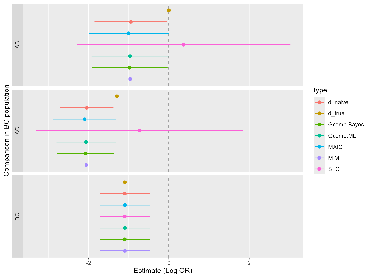
We now combine all outputs and present in plots and tables. For a log-odds ratio a table of all contrasts and methods in the $BC$ population is given below.

	d_true	d_naive	MAIC	STC	Gcomp.ML	Gcomp.Bayes	MIM
AB	0.00	-0.95	-1.0	-1.12	-0.97	-0.99	-0.99
AC	-1.29	-2.05	-2.1	-2.21	-2.06	-2.08	-2.09
BC	-1.10	-1.10	-1.1	-1.10	-1.10	-1.10	-1.10

We can see that the different corresponds reasonably well with one another.

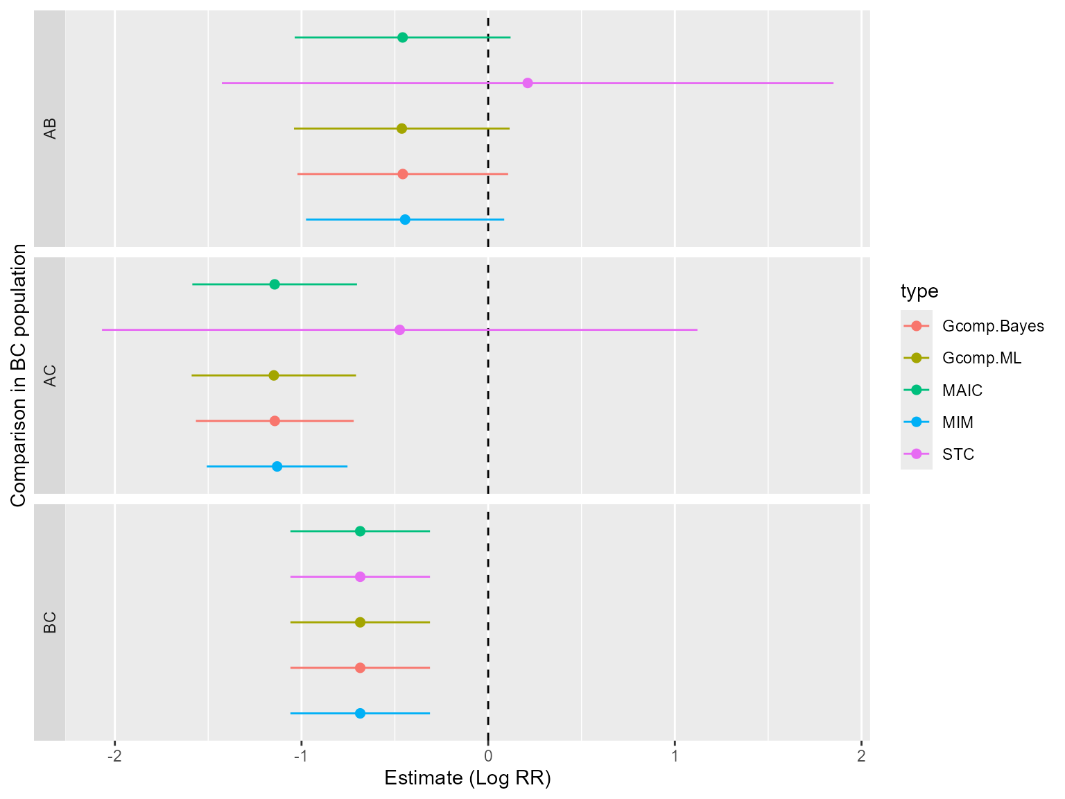
Next, let us look at the results on the log relative risk scale. First, the true values are calculated as

d_AB_true_lrr <- 0
d_AC_true_lrr <- log(plogis(d_A_true) / plogis(d_C_true))
d_AC_true_lrr

so that the summary table is

	MAIC	STC	Gcomp.ML	Gcomp.Bayes	MIM
AB	-0.46	-0.72	-0.46	-0.46	-0.46
AC	-1.14	-1.40	-1.15	-1.14	-1.14
BC	-0.69	-0.69	-0.69	-0.69	-0.69

Plots

The same output can be presented in forest plots is as follows. Each horizontal bar represent a different method and the facets group these by treatment comparison for the $BC$ population. The log-odds ratio and log risk ratio plot are given below.