Checkmate 067 study Bayesian mixture cure model analysis
Nathan Green, Gianluca Baio, UCL
02 April, 2021
Check_mate_analysis.RmdExecutive summary
In this project we formulate and demonstrate the application of a Bayesian mixture cure model (MCM) using the Checkmate 067 study dataset for a range of survival distributions. Analogous results to those created previously for the frequentist MCM approach are produced and we extend the Bayesian MCM to incorporate additional structure. This includes modelling the cure fractions separately for OS and PFS (as in the frequentist approach) and by joining the overall survival (OS) and progression-free survival (PFS) models using a hierarchical (multilevel) structure on the cure fraction. We show that the Exponential and in particular the log-logistic OS and PFS Bayesian MCMs perform reasonably well for the Checkmate 067 data. We also perform a sensitivity analysis by increasing the background hazard rate via a hazard ratio adjustment, representing a study population with a higher mortality rate than the general population. The real benefit of this approach, not full explored in this analysis, may be with other dataset where there is relatively short follow-up or small sample sizes. The associated R code for this work, held in a private on-line repository, has been written for re-use and generalisability to other problems.
Background
Immuno-oncologic (IO) studies for melanoma therapies, such as ipilimumab (ipi), nivolumab (nivo), and the nivolumab with ipilimumab (nivo + ipi) combination, have indicated that survival curves “plateau” (a considerable proportion of patients are “long-term survivors”). Cure models are a special type of survival analysis where this “cure fraction” (the underlying proportion of responders to treatment/long-term survivors) is accounted for. Cure models estimate the cure fraction, in addition to a parametric survival function for patients that are not cured. The mortality risk in the cured patients is informed by a background mortality rate. The population that is not cured is subject both to background mortality and to additional mortality from their cancer, estimated using a parametric survival model.
A mixture cure model (MCM) (Amico and Van Keilegom (2018)) is a type of cure model where survival is modelled as a mixture of two groups of patients: those who are cured and those who are not (and who therefore remain at risk). The survival for a population with a cure fraction can be written as follows:
\[\begin{align} \tag{*} S(t, x) = S^*(t, x)[\pi(x) + (1 − \pi(x))S_u(t, x)], \end{align}\]where \(S(t, x)\) denotes the survival at time \(t\), \(S^*(t, x)\) denotes the background mortality at time \(t\) conditional on covariates \(x\), \(\pi(x)\) denotes the probability of being cured conditional on covariates \(x\), and \(S_u(t, x)\) denotes the event (progression or mortality) due to cancer at time \(t\) conditional on covariates \(x\). For PFS, the survival is composed of either progressing to a disease state or death.
Aims
The aims of the the analysis in this document are as follows:
- Demonstrate the application of a Bayesian mixture cure model using the Checkmate 067 study dataset and the Exponential distribution for event times.
- Produce analogous results to those created previously for the frequentist approach.
- Extend the Bayesian model to incorporate additional structure including a hierarchical cure fraction.
This analysis has been carried-out using the Stan inference engine (Carpenter et al. (2017)) called from R on a Windows PC. The packaged code can be downloaded from a private GitHub repository with permission from the package authors at https://github.com/StatisticsHealthEconomics/rstanbmcm. See the How to use rstanbmcm vignette for an introduction to how to use the package.
Likelihood
Let \(T_i\) be the non-negative random variable denoting the survival time of patient \(i\) with covariate vector \(\boldsymbol{x}_i\).
In the simplest case we can assume that the cure fraction is the same for the whole population i.e. \(\pi\) is fixed. Further, we can assume the \(\pi\) models the relationship between \(\boldsymbol{x}_i\) and the probability of being cured. E.g. using a logistic-linear model
\[ \pi(\boldsymbol{x}_i | \boldsymbol{\beta}) = 1/[1 + \exp(-\boldsymbol{x}_i^T \boldsymbol{\beta})]. \]
The likelihood of the standard survival is
\[ L = \prod_i S(t_i | \boldsymbol{x}_i) h(t_i | \boldsymbol{x}_i)^{\delta_i} \]
Log-likelihood is therefore \[ \mathcal{l} = \sum_i \log(S(t_i | \boldsymbol{x}_i)) + \delta_i \log(h(t_i | \boldsymbol{x}_i)) \]
Plugging this directly into the mixture cure equation in (*) gives
\[ \mathcal{l}(\pi | \boldsymbol{\delta}, \boldsymbol{x}) = \sum_i \log(S^*(t_i | \boldsymbol{x}_i) h^*(t_i | \boldsymbol{x}_i)^{\delta_i}[\pi(x) + (1 − \pi(x)) S_u(t_i | \boldsymbol{x}_i) h_u(t_i | \boldsymbol{x}_i)^{\delta_i}]) \]
If we assume that the cured component is the Exponential survival model then the non-cured component can be thought of in similar terms to the cumulative incidence function. That is, the probability of an event is the combined probability of surviving both events (e.g. for OS, all-cause and cancer mortality) and then experiencing either i.e. dropping the \(S\) dependencies for brevity
\[\begin{equation} \tag{**} S^* S_u (h^*)^{\delta} + S^* S_u (h_u)^{\delta} = S^* S_u (h^* + h_u)^{\delta} \end{equation}\]Bayesian formulation
In a Bayesian approach to modelling (McElreath (2018)), all quantities that are subject to uncertainty are modelled using probability distributions. This applies to observed data (e.g. time to PFS for a given individual), that are subject to sampling variability, as well as to unobservable parameters (e.g. the coefficient quantifying the impact of age or sex over the average survival curve). In this latter case, probability distributions are used to model the epistemic uncertainty (e.g. the fact that we do not know for certain what the “true” underlying value of the model parameter is). In addition, we may model as yet unobserved (but potentially observable) quantities using a suitable probability model. For example, we could consider the extrapolated part of the survival curve as subject to uncertainty due to the current sampling process giving rise to the data that are actually observed, as well as the uncertainty on the underlying data generating process.
We can mix different sources of evidence to form our “prior” distributions, which are used to describe the state of science on the model parameters. These are then combined with any observed data to form an updated level of knowledge. This process is particularly relevant in the case at hand, when data can only inform about limited aspects of the overall underlying reality. For this reason, it is important to a) include information/evidence available in the form of external data and/or expert opinion; b) extract the most information possible from the available data (e.g. by formally trying to model the correlation between the PFS and the OS data to borrow strength from the more mature set of observations).
A built-in advantage of the Bayesian procedure is that uncertainty is directly and formally propagated to an economic model; the main output from the statistical analysis (the extrapolated survival curve) are produced by default as based on a full posterior distribution. From this, we can easily derive a “base case” (e.g. taking the mean value) but without the need for further tools (such as bootstrap) we already have a full characterisation of the underlying uncertainty that can be used in the process of probabilistic sensitivity analysis. We can moreover add information in the priors to ensure that the extrapolation beyond the observed data is realistic and consistent with the clinical expertise (e.g. by “anchoring” the extrapolated survival curve to be probabilistically below the curves for the healthy population, or by ensuring that OS behaves in a way to respect some agreed level of similarity, or correlation, to PFS).
Posterior equation
Using the likelihood function defined above and prior distributions on uncertain parameters, we can specify the posterior distribution. Defining \(g_2\) as the prior distribution for the coefficients of the uncured fraction \(\beta^u\) and \(g_3\) as the prior distribution for the coefficients of the cured fraction \(\beta^*\), then the general form of the posterior distribution can be written as follows.
\[ p(\pi, \boldsymbol{\beta^u}, \boldsymbol{\beta^*} | \boldsymbol{\delta}, \boldsymbol{x}) \propto L(\pi, \boldsymbol{\beta^u}, \boldsymbol{\beta^*} | \boldsymbol{\delta}, \boldsymbol{x}) f(\pi) g_2(\boldsymbol{\beta^u}) g_3(\boldsymbol{\beta^*}) \]
assuming that the cure fraction is independent of the covariates.
Cure fraction
There are two obvious ways to represent the uncertainty about the cure fraction in the model.
The first is to specify the cure fraction directly using a \(\pi \sim Beta(a_{cf}, b_{cf})\) prior, most uninformative as a uniform \(Beta(1,1)\). The parameters can be obtained via transformation of mean and standard deviation to allow a more natural scale for elicitation.
Alternatively, we may specify the uncertainty on the real line with a Normal distribution and then transform to the probability scale.
A further consideration is how to represent the cure fraction so to share information between the OS and PFS data. We will investigate 3 alternatives.
- Pooled: Assume that the cure fraction is the same for OS and PFS i.e. \(\pi_{os} = \pi_{os} = \pi\) where \[ logit(\pi) \sim N(\mu_{cf}, \sigma_{cf}^2), \;\; \]
- Separate: Model each independently. \[ logit(\pi_{os}) \sim N(\mu_{cfos}, \sigma_{cfos}^2), \;\; logit(\pi_{pfs}) \sim N(\mu_{cfpfs}, \sigma_{cfpfs}^2) \]
- Hierarchical: Assume exchangeability between OS and PFS\[ \pi \sim N(\mu_{cf}, \sigma_{cf}^2), \;\; logit(\pi_{os}) \sim N(\pi, \sigma_{cfos}^2), \;\; logit(\pi_{pfs}) \sim N(\pi, \sigma_{cfpfs}^2) \]
Below is an example DAG for the hierarchical cure fraction without a joint time to event component. Notice that even without the direct relationship between PFS and OS there is still an indirect influence via \(\pi\).
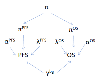
Hierarchical cure fraction DAG.
Background survival
The previous frequentist analysis used the World Health Organization (WHO) life tables by country for the latest year available of 2016 (WHO (2020)) to inform the background mortality rate (baseline hazard). These baseline hazards are the expected mortality rate for each patient at the age at which they experience the event. The mortality data are age- and gender adjusted, thus providing a granular account of the different patient profiles in the trial. The WHO reports conditional probabilities of death in 5-year intervals until age 85. A constant annual mortality rate is reported for individuals over 85. They assumed that the maximum age is 100 years.
In a Bayesian analysis there are alternative ways in which we could model the background mortality.
For this work we shall use WHO hazard point estimates as known. We could consider the WHO estimates to provide sufficiently accurate estimates given the sample size and so incorporating uncertainty is not necessary. This also forces consistency across fits. Denote the WHO estimates for individual \(i\) as \(\hat{f}_i, \hat{S}_i, \hat{h}_i\) for the density, survival and hazard respectively.
This gives the likelihood
\[ L(\pi | \boldsymbol{\delta}, \boldsymbol{x}, \hat{S}, \hat{h}) = \sum_i \hat{S}_i \hat{h}_i^{\delta_i} \left[ \pi(x) + (1 - \pi(x)) S_{u, i} h_{u , i}^{\delta_i} \right] \]
Results
We fit the separate and exchangeable cure fraction models to the study data and produced the posterior survival curves below.
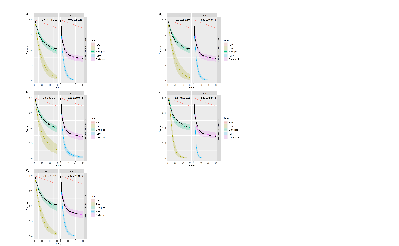
For each model and treatment we produce the expected survival curves with 95% Credible Intervals (CrI). The OS curves are to the left-hand side and PFS curves to the right-hand side. Background mortality (i.e. cured patients) is indicated by the red line. Non-cured patients survival curves are shown in dark green and blue for OS and PFS respectively. Light green and magenta are the total sample. The black line is the Kaplan-Meier curve for the observed data. Note that these plots are for an average individual, e.g. at average age, and so we would not expect them to perfectly match the sample data Kaplan-Meier.
Separate survival models for OS and PFS
Figures , , and show posterior survival curves for the Exponential, log-logistic, Gompertz, Weibull and log-Normal models when the OS and PFS models are fitted separately.
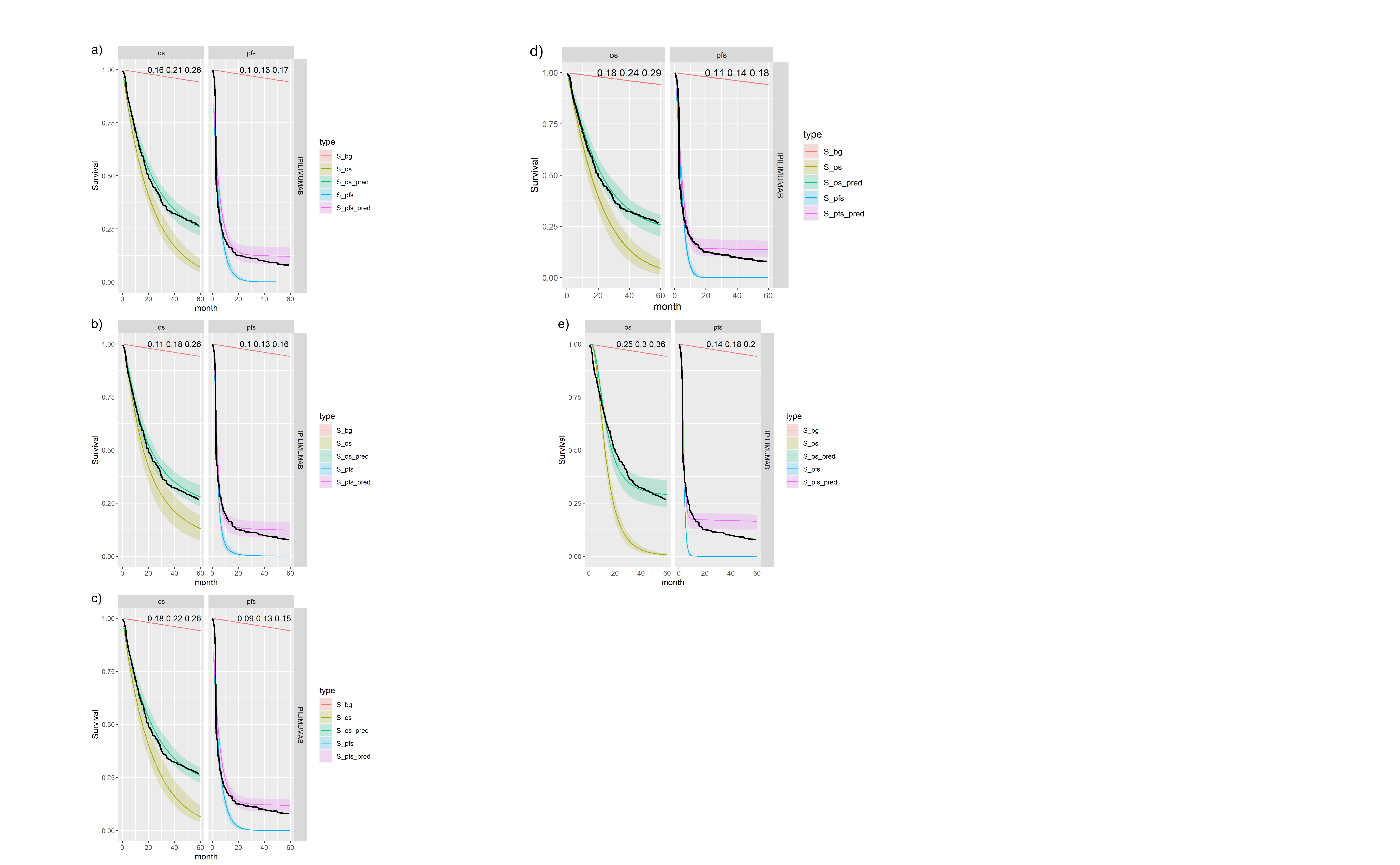
Posterior survival curves for the mixture cure model for separate OS and PFS models and \(ipilimumab\). The red line is cured background, light green and blue are uncured, and dark green and magenta are combined. a) Exponential uncured b) Log-logistic uncured c) Gompertz uncured d) Weibull uncured e) Log-Normal uncured.

Posterior survival curves for the mixture cure model for separate OS and PFS models and \(nivolumab\). The red line is cured background, light green and blue are uncured, and dark green and magenta are combined. a) Exponential uncured b) Log-logistic uncured c) Gompertz uncured d) Weibull uncured e) Log-Normal uncured.
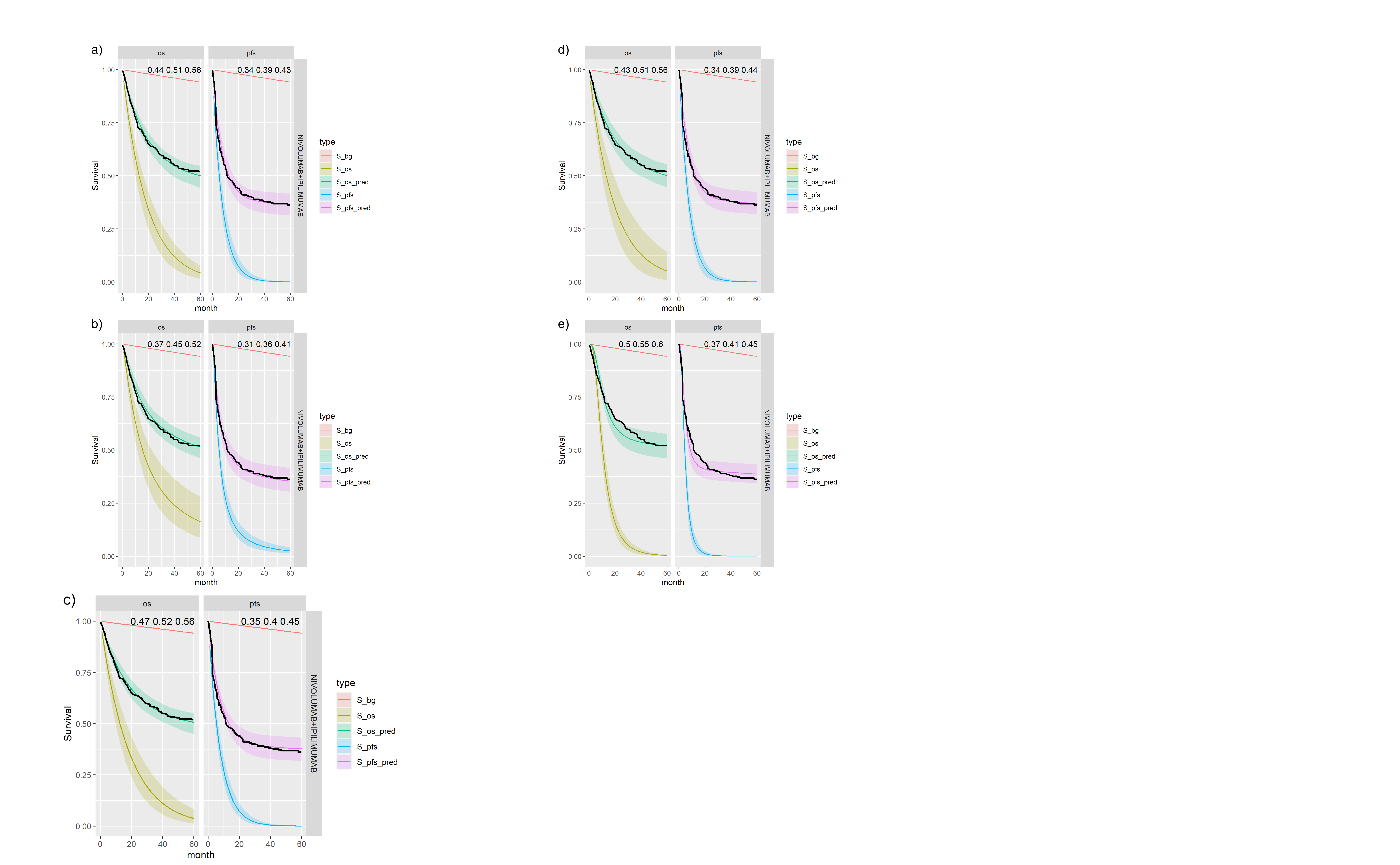
Posterior survival curves for the mixture cure model for separate OS and PFS models and \(ipilimumab\) and \(nivolumab\). The red line is cured background, light green and blue are uncured, and dark green and magenta are combined. a) Exponential uncured b) Log-logistic uncured c) Gompertz uncured d) Weibull uncured e) Log-Normal uncured.
Figures and show the forest plots of cure fraction posterior distributions.
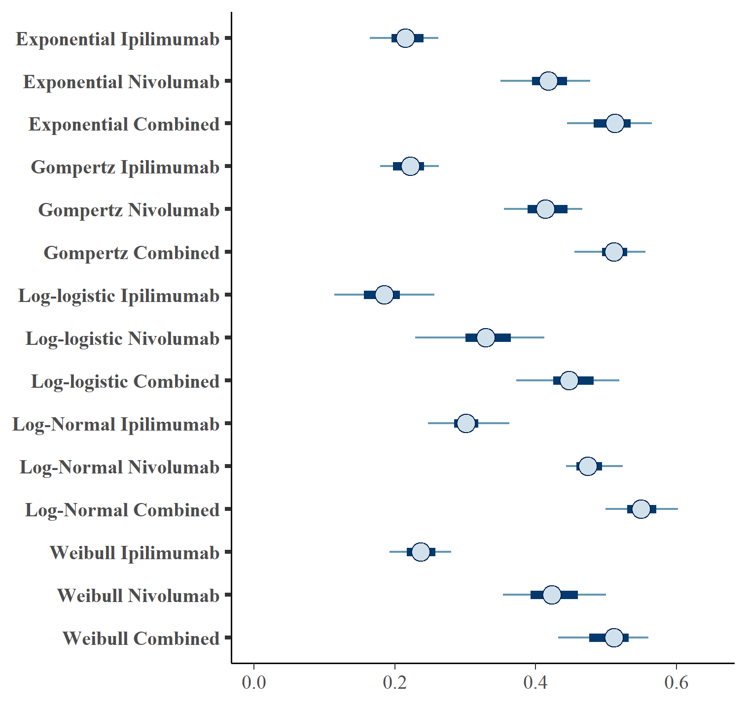
Forest plot of OS cure fraction posterior distributions for separate OS and PFS models .
Forest plot of PFS cure fraction posterior distributions for separate OS and PFS models .
| OS Distn | PFS Distn | Treatment | \(cf_{OS}\) (CrI) | \(cf_{PFS}\) (CrI) | |
|---|---|---|---|---|---|
| 1 | exp | exp | IPILIMUMAB | 0.216 (0.16, 0.271) | 0.128 (0.089, 0.173) |
| 2 | exp | exp | NIVOLUMAB | 0.417 (0.335, 0.482) | 0.32 (0.268, 0.37) |
| 3 | exp | exp | NIVOLUMAB+IPILIMUMAB | 0.509 (0.43, 0.573) | 0.387 (0.332, 0.441) |
| 4 | gompertz | gompertz | IPILIMUMAB | 0.221 (0.176, 0.282) | 0.126 (0.092, 0.156) |
| 5 | gompertz | gompertz | NIVOLUMAB | 0.414 (0.352, 0.477) | 0.321 (0.274, 0.383) |
| 6 | gompertz | gompertz | NIVOLUMAB+IPILIMUMAB | 0.51 (0.447, 0.575) | 0.39 (0.323, 0.457) |
| 7 | loglogistic | loglogistic | IPILIMUMAB | 0.183 (0.11, 0.265) | 0.13 (0.091, 0.168) |
| 8 | loglogistic | loglogistic | NIVOLUMAB | 0.329 (0.217, 0.423) | 0.321 (0.267, 0.381) |
| 9 | loglogistic | loglogistic | NIVOLUMAB+IPILIMUMAB | 0.449 (0.349, 0.524) | 0.359 (0.308, 0.427) |
| 10 | lognormal | lognormal | IPILIMUMAB | 0.304 (0.241, 0.378) | 0.175 (0.13, 0.207) |
| 11 | lognormal | lognormal | NIVOLUMAB | 0.477 (0.432, 0.531) | 0.424 (0.375, 0.467) |
| 12 | lognormal | lognormal | NIVOLUMAB+IPILIMUMAB | 0.55 (0.487, 0.611) | 0.411 (0.365, 0.459) |
| 13 | weibull | weibull | IPILIMUMAB | 0.238 (0.177, 0.285) | 0.146 (0.105, 0.186) |
| 14 | weibull | weibull | NIVOLUMAB | 0.425 (0.348, 0.51) | 0.317 (0.261, 0.378) |
| 15 | weibull | weibull | NIVOLUMAB+IPILIMUMAB | 0.504 (0.423, 0.566) | 0.392 (0.339, 0.45) |
The table below gives the leave-one-out cross validation statistics for each model fit using WAIC (Vehtari, Gelman, and Gabry (2017)).
| OS Distn | PFS Distn | Treatment | Statistic | Estimate | SE |
|---|---|---|---|---|---|
| exp | exp | IPILIMUMAB | elpd_waic | -1548.19 | 53.04 |
| exp | exp | NIVOLUMAB | elpd_waic.1 | -1548.57 | 53.21 |
| exp | exp | NIVOLUMAB+IPILIMUMAB | elpd_waic.2 | -1541.23 | 52.74 |
| gompertz | gompertz | IPILIMUMAB | elpd_waic.3 | -1487.44 | 57.45 |
| gompertz | gompertz | NIVOLUMAB | elpd_waic.4 | -1549.41 | 53.59 |
| gompertz | gompertz | NIVOLUMAB+IPILIMUMAB | p_waic | 6.05 | 0.61 |
| loglogistic | loglogistic | IPILIMUMAB | p_waic.1 | 6.59 | 0.53 |
| loglogistic | loglogistic | NIVOLUMAB | p_waic.2 | 7.69 | 0.53 |
| loglogistic | loglogistic | NIVOLUMAB+IPILIMUMAB | p_waic.3 | 14.76 | 1.22 |
| lognormal | lognormal | IPILIMUMAB | p_waic.4 | 7.92 | 0.72 |
| lognormal | lognormal | NIVOLUMAB | waic | 3096.38 | 106.09 |
| lognormal | lognormal | NIVOLUMAB+IPILIMUMAB | waic.1 | 3097.14 | 106.41 |
| weibull | weibull | IPILIMUMAB | waic.2 | 3082.45 | 105.49 |
| weibull | weibull | NIVOLUMAB | waic.3 | 2974.89 | 114.90 |
| weibull | weibull | NIVOLUMAB+IPILIMUMAB | waic.4 | 3098.82 | 107.17 |
Exchangeable cure fraction for OS and PFS
Figures , , and show posterior survival curves for the Exponential, log-logistic, Gompertz, Weibull and log-Normal models when the OS and PFS models share information with exchangeable cure fractions.
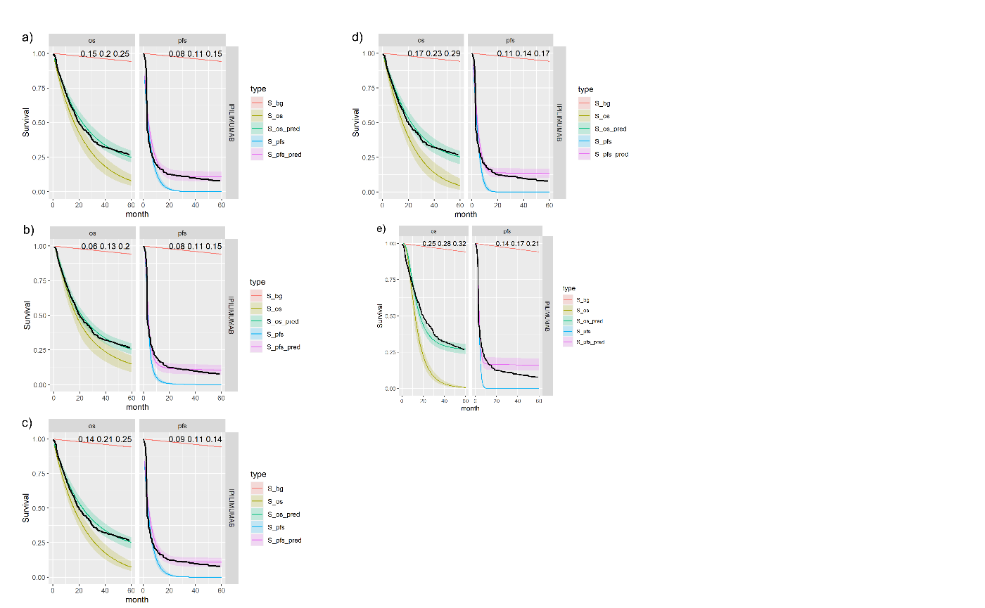
Posterior survival curves for the mixture cure model with exchangeable cure fracion and \(ipilimumab\). The red line is cured background, light green and blue are uncured, and dark green and magenta are combined. a) Exponential uncured b) Log-logistic uncured c) Gompertz uncured d) Weibull uncured e) Log-Normal uncured.
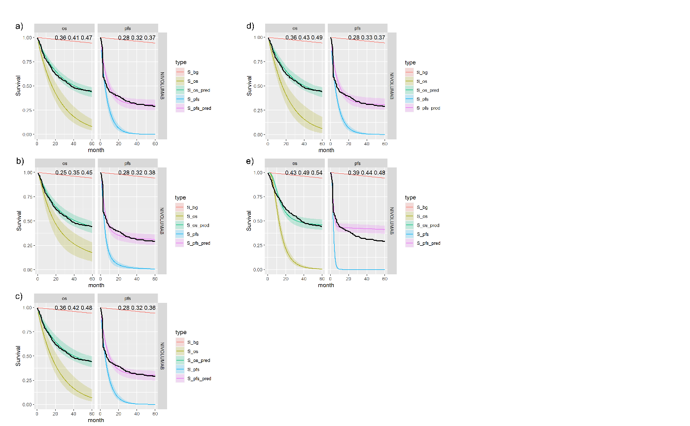
Posterior survival curves for the mixture cure model with exchangeable cure fracion and \(nivolumab\). The red line is cured background, light green and blue are uncured, and dark green and magenta are combined. a) Exponential uncured b) Log-logistic uncured c) Gompertz uncured d) Weibull uncured e) Log-Normal uncured.
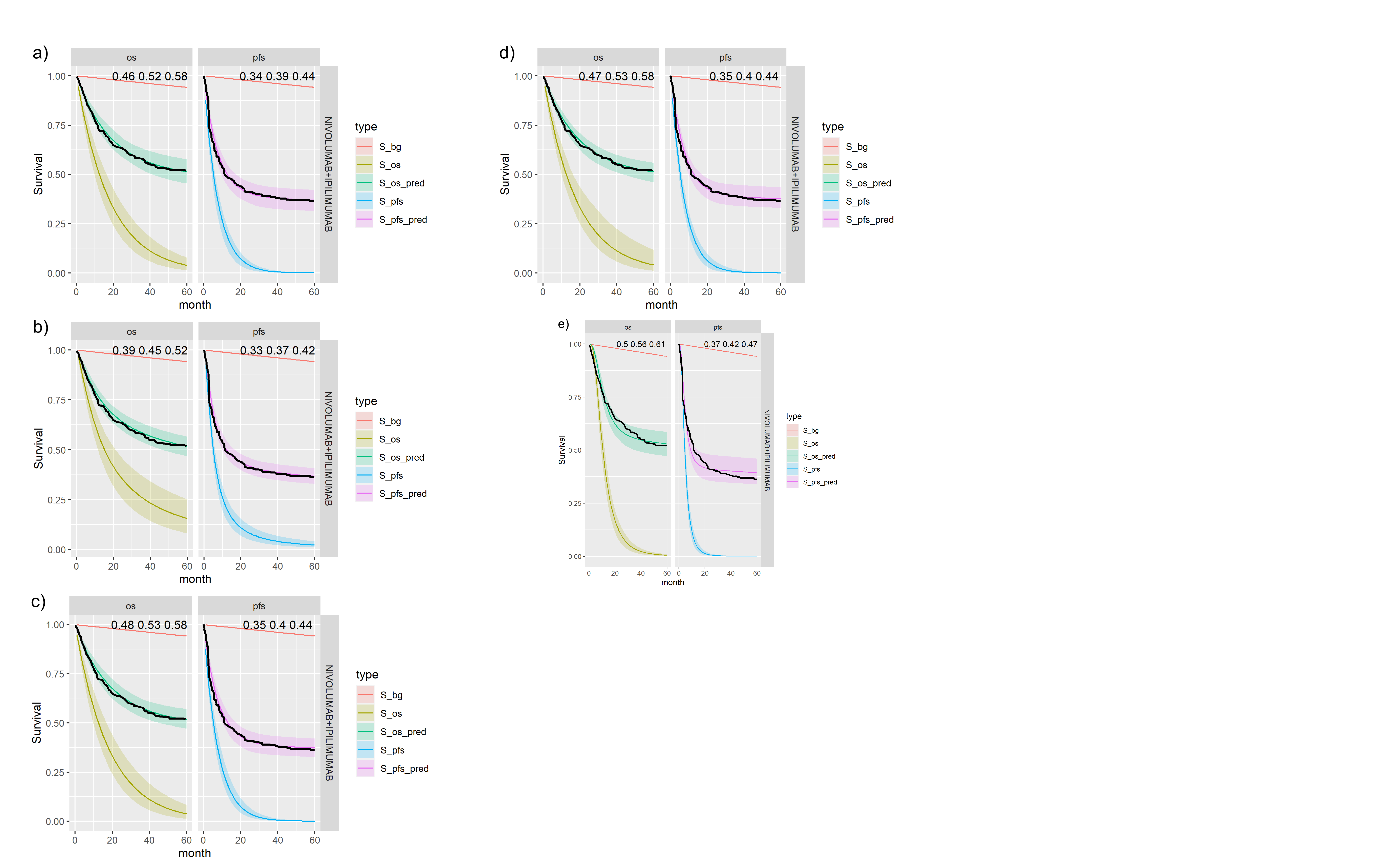
Posterior survival curves for the mixture cure model with exchangeable cure fracion and dual \(ipilimumab\) and \(nivolumab\). The red line is cured background, light green and blue are uncured, and dark green and magenta are combined. a) Exponential uncured b) Log-logistic uncured c) Gompertz uncured d) Weibull uncured e) Log-Normal uncured.
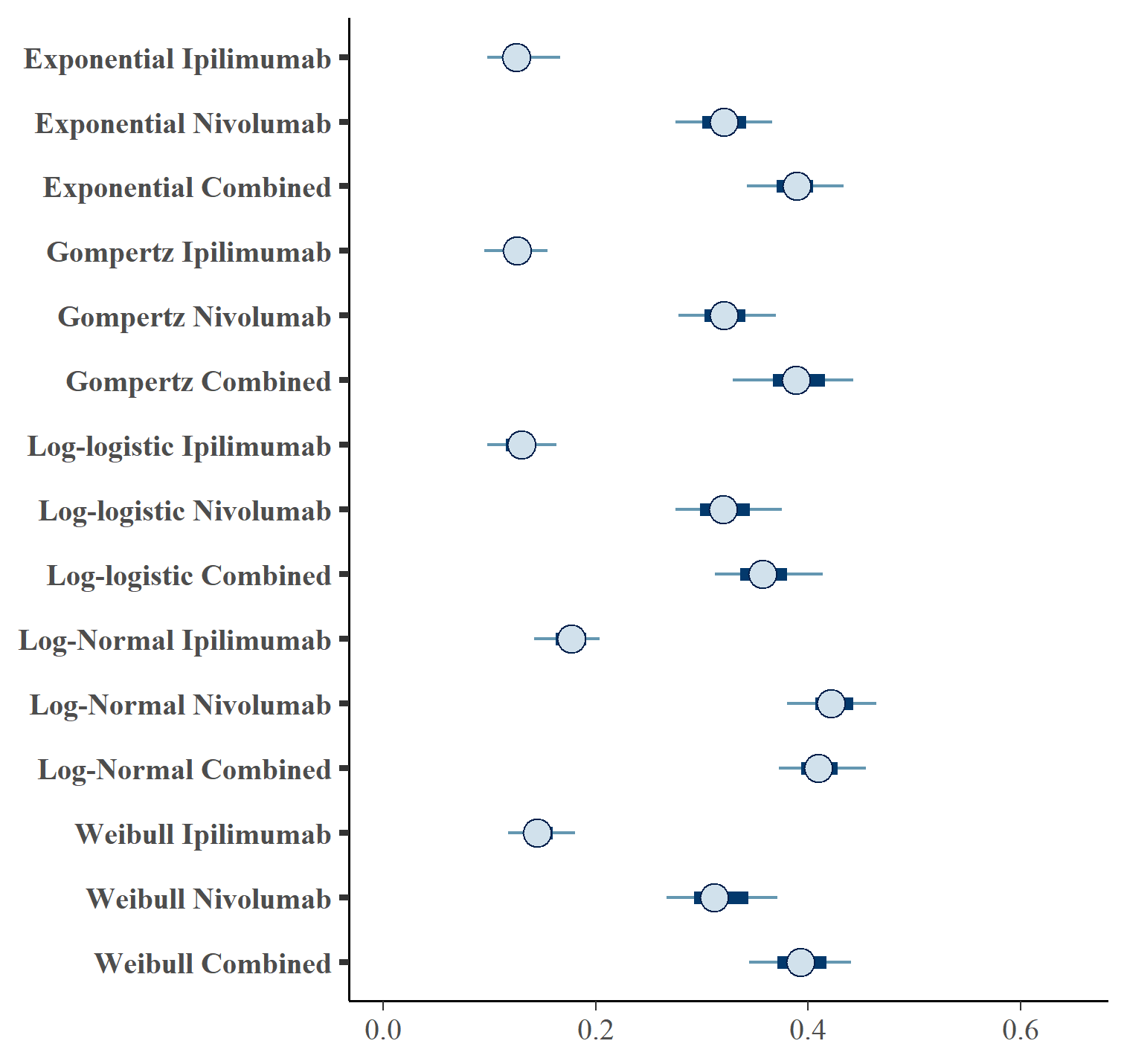
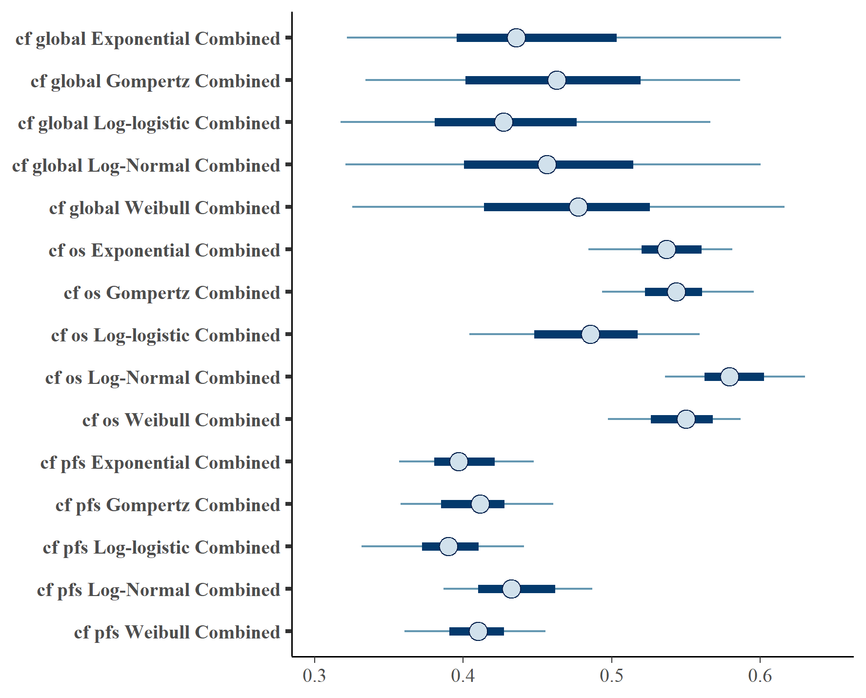
Figures , and show the forest plots of cure fraction posterior distributions. We see that the values are generally similar for the Exponential and log-logistic fits. This clearly shows how the global cure fraction posterior distribution lies partway between the PFS and OS distributions.
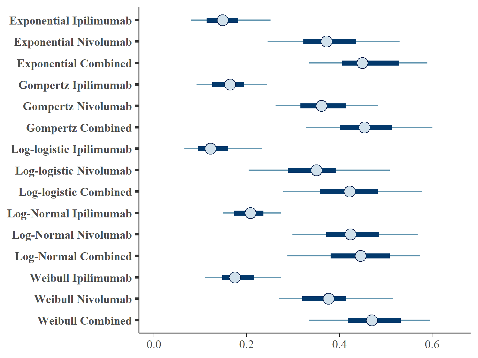
Forest plot of global cure fraction posterior distributions.
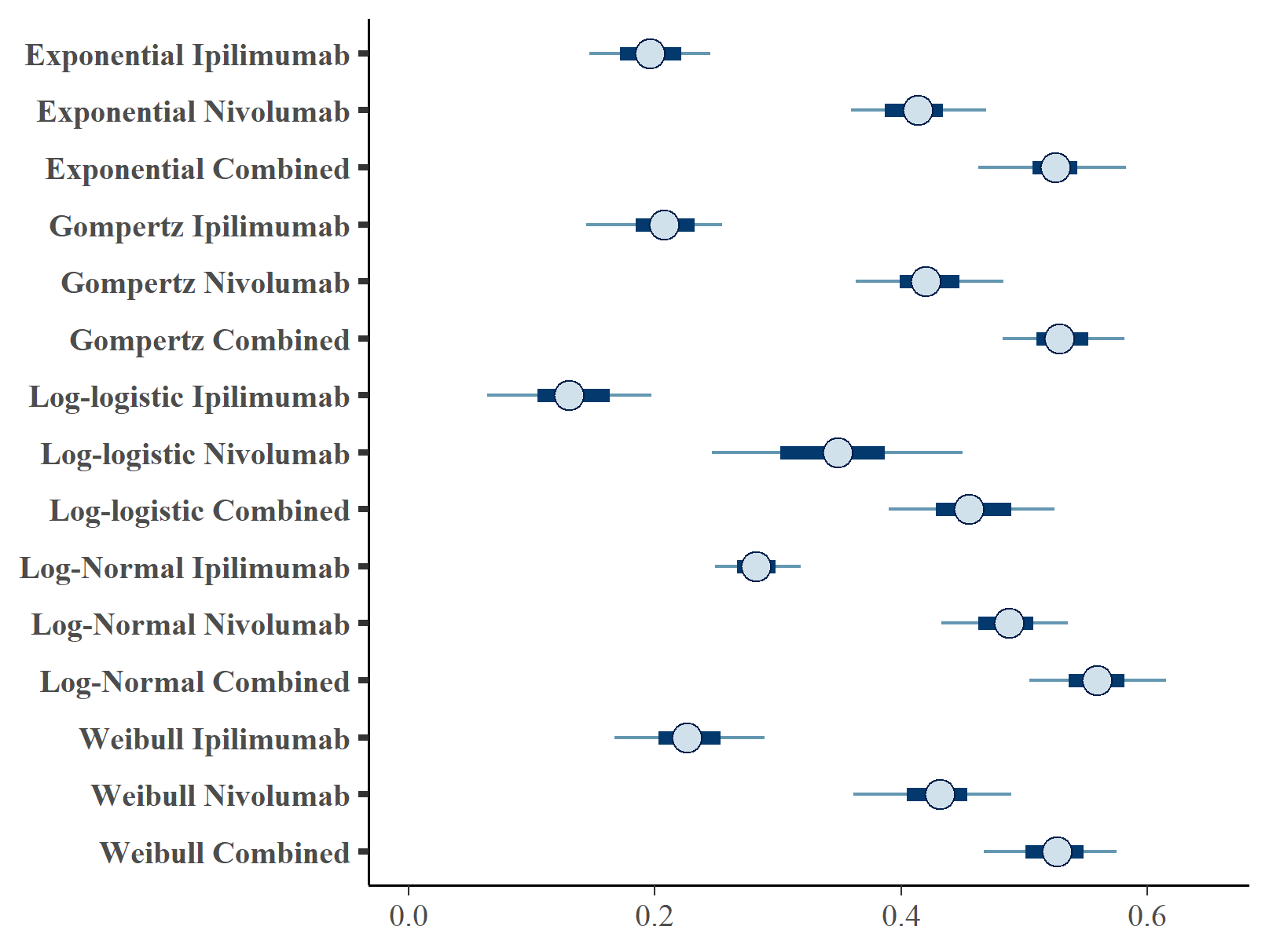
Forest plot of OS cure fraction posterior distributions.
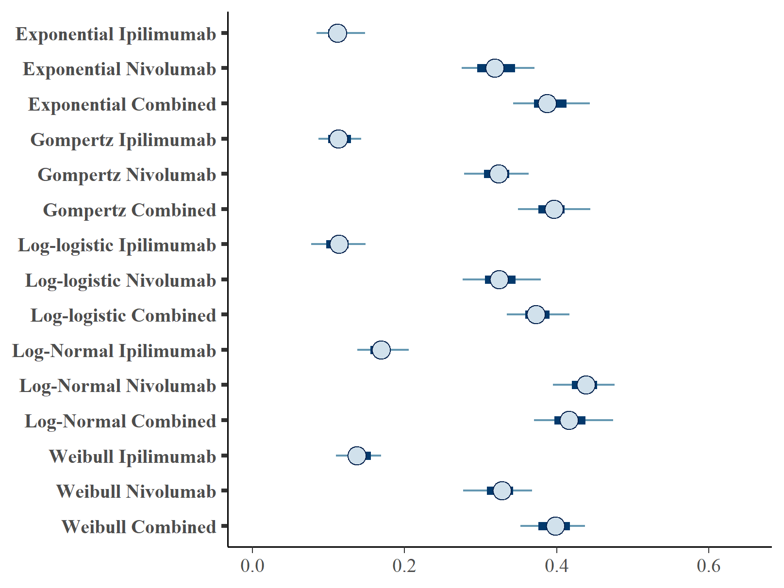
Forest plot of PFS cure fraction posterior distributions.
The table below summarises the cure fraction posterior distribution for each scenario.
| OS Distn | PFS Distn | Treatment | \(cf\) (CrI) | \(cf_{OS}\) (CrI) | \(cf_{PFS}\) (CrI) | |
|---|---|---|---|---|---|---|
| 1 | exp | exp | IPILIMUMAB | 0.151 (0.068, 0.26) | 0.196 (0.136, 0.255) | 0.112 (0.079, 0.155) |
| 2 | exp | exp | NIVOLUMAB | 0.378 (0.216, 0.557) | 0.412 (0.35, 0.479) | 0.321 (0.262, 0.379) |
| 3 | exp | exp | NIVOLUMAB+IPILIMUMAB | 0.463 (0.328, 0.626) | 0.526 (0.452, 0.597) | 0.392 (0.334, 0.448) |
| 4 | gompertz | gompertz | IPILIMUMAB | 0.164 (0.088, 0.275) | 0.207 (0.13, 0.266) | 0.114 (0.079, 0.148) |
| 5 | gompertz | gompertz | NIVOLUMAB | 0.368 (0.247, 0.517) | 0.423 (0.358, 0.494) | 0.321 (0.261, 0.369) |
| 6 | gompertz | gompertz | NIVOLUMAB+IPILIMUMAB | 0.458 (0.318, 0.612) | 0.529 (0.477, 0.594) | 0.395 (0.346, 0.446) |
| 7 | loglogistic | loglogistic | IPILIMUMAB | 0.133 (0.061, 0.278) | 0.133 (0.054, 0.206) | 0.113 (0.075, 0.152) |
| 8 | loglogistic | loglogistic | NIVOLUMAB | 0.348 (0.191, 0.526) | 0.345 (0.231, 0.456) | 0.325 (0.264, 0.382) |
| 9 | loglogistic | loglogistic | NIVOLUMAB+IPILIMUMAB | 0.421 (0.266, 0.599) | 0.459 (0.37, 0.535) | 0.375 (0.327, 0.421) |
| 10 | lognormal | lognormal | IPILIMUMAB | 0.236 (0.127, 0.303) | 0.285 (0.198, 0.468) | 0.177 (0.136, 0.293) |
| 11 | lognormal | lognormal | NIVOLUMAB | 0.425 (0.286, 0.588) | 0.486 (0.431, 0.546) | 0.437 (0.39, 0.48) |
| 12 | lognormal | lognormal | NIVOLUMAB+IPILIMUMAB | 0.431 (0.301, 0.581) | 0.556 (0.494, 0.619) | 0.42 (0.37, 0.481) |
| 13 | weibull | weibull | IPILIMUMAB | 0.184 (0.095, 0.29) | 0.229 (0.157, 0.295) | 0.141 (0.107, 0.177) |
| 14 | weibull | weibull | NIVOLUMAB | 0.375 (0.242, 0.541) | 0.427 (0.346, 0.494) | 0.326 (0.27, 0.394) |
| 15 | weibull | weibull | NIVOLUMAB+IPILIMUMAB | 0.471 (0.328, 0.647) | 0.523 (0.461, 0.58) | 0.399 (0.35, 0.462) |
The table below gives the leave-one-out cross validation statistics for each model fit.
| OS Distn | PFS Distn | Treatment | Statistic | Estimate | SE |
|---|---|---|---|---|---|
| exp | exp | IPILIMUMAB | elpd_waic | -1838.83 | 36.07 |
| exp | exp | NIVOLUMAB | elpd_waic | -1679.59 | 45.69 |
| exp | exp | NIVOLUMAB+IPILIMUMAB | elpd_waic | -1549.68 | 60.15 |
| gompertz | gompertz | IPILIMUMAB | elpd_waic | -1488.81 | 58.20 |
| gompertz | gompertz | NIVOLUMAB | elpd_waic | -1819.89 | 39.69 |
| gompertz | gompertz | NIVOLUMAB+IPILIMUMAB | elpd_waic | -1680.25 | 45.91 |
| loglogistic | loglogistic | IPILIMUMAB | elpd_waic | -1544.04 | 54.19 |
| loglogistic | loglogistic | NIVOLUMAB | elpd_waic | -1543.49 | 53.87 |
| loglogistic | loglogistic | NIVOLUMAB+IPILIMUMAB | elpd_waic | -1839.34 | 36.27 |
| lognormal | lognormal | IPILIMUMAB | elpd_waic | -1679.48 | 45.80 |
| lognormal | lognormal | NIVOLUMAB | elpd_waic | -1543.81 | 54.03 |
| lognormal | lognormal | NIVOLUMAB+IPILIMUMAB | elpd_waic | -1768.17 | 39.20 |
| weibull | weibull | IPILIMUMAB | elpd_waic | -1651.73 | 46.02 |
| weibull | weibull | NIVOLUMAB | elpd_waic | -1533.95 | 53.17 |
| weibull | weibull | NIVOLUMAB+IPILIMUMAB | elpd_waic | -1566.33 | 55.91 |
| exp | exp | IPILIMUMAB | p_waic | 5.37 | 0.48 |
| exp | exp | NIVOLUMAB | p_waic | 7.45 | 0.62 |
| exp | exp | NIVOLUMAB+IPILIMUMAB | p_waic | 15.46 | 1.44 |
| gompertz | gompertz | IPILIMUMAB | p_waic | 14.55 | 1.26 |
| gompertz | gompertz | NIVOLUMAB | p_waic | 9.46 | 0.96 |
| gompertz | gompertz | NIVOLUMAB+IPILIMUMAB | p_waic | 8.70 | 0.75 |
| loglogistic | loglogistic | IPILIMUMAB | p_waic | 7.70 | 0.72 |
| loglogistic | loglogistic | NIVOLUMAB | p_waic | 7.15 | 0.60 |
| loglogistic | loglogistic | NIVOLUMAB+IPILIMUMAB | p_waic | 5.91 | 0.52 |
| lognormal | lognormal | IPILIMUMAB | p_waic | 6.96 | 0.56 |
| lognormal | lognormal | NIVOLUMAB | p_waic | 7.07 | 0.78 |
| lognormal | lognormal | NIVOLUMAB+IPILIMUMAB | p_waic | 9.19 | 0.56 |
| weibull | weibull | IPILIMUMAB | p_waic | 9.20 | 0.53 |
| weibull | weibull | NIVOLUMAB | p_waic | 6.10 | 0.50 |
| weibull | weibull | NIVOLUMAB+IPILIMUMAB | p_waic | 20.04 | 1.20 |
| exp | exp | IPILIMUMAB | waic | 3677.65 | 72.13 |
| exp | exp | NIVOLUMAB | waic | 3359.19 | 91.37 |
| exp | exp | NIVOLUMAB+IPILIMUMAB | waic | 3099.36 | 120.30 |
| gompertz | gompertz | IPILIMUMAB | waic | 2977.62 | 116.41 |
| gompertz | gompertz | NIVOLUMAB | waic | 3639.77 | 79.38 |
| gompertz | gompertz | NIVOLUMAB+IPILIMUMAB | waic | 3360.49 | 91.83 |
| loglogistic | loglogistic | IPILIMUMAB | waic | 3088.08 | 108.39 |
| loglogistic | loglogistic | NIVOLUMAB | waic | 3086.98 | 107.74 |
| loglogistic | loglogistic | NIVOLUMAB+IPILIMUMAB | waic | 3678.68 | 72.53 |
| lognormal | lognormal | IPILIMUMAB | waic | 3358.96 | 91.59 |
| lognormal | lognormal | NIVOLUMAB | waic | 3087.62 | 108.05 |
| lognormal | lognormal | NIVOLUMAB+IPILIMUMAB | waic | 3536.33 | 78.40 |
| weibull | weibull | IPILIMUMAB | waic | 3303.47 | 92.04 |
| weibull | weibull | NIVOLUMAB | waic | 3067.91 | 106.35 |
| weibull | weibull | NIVOLUMAB+IPILIMUMAB | waic | 3132.66 | 111.82 |
The variance partition coefficient (VPC) is defined as \(\sigma_{global}^2/ (\sigma_{global}^2 + \sigma_{e}^2)\) where \(e = PFS\) or \(OS\). This indicates want proportion of the total variance is attributable to variation within-groups, or how much is found between-groups.
| OS Distn | PFS Distn | Treatment | PFS | OS |
|---|---|---|---|---|
| exp | exp | IPILIMUMAB | 0.813 | 0.784 |
| exp | exp | NIVOLUMAB | 0.876 | 0.877 |
| exp | exp | NIVOLUMAB+IPILIMUMAB | 0.865 | 0.860 |
| gompertz | gompertz | IPILIMUMAB | 0.781 | 0.743 |
| gompertz | gompertz | NIVOLUMAB | 0.858 | 0.808 |
| gompertz | gompertz | NIVOLUMAB+IPILIMUMAB | 0.899 | 0.888 |
| loglogistic | loglogistic | IPILIMUMAB | 0.812 | 0.604 |
| loglogistic | loglogistic | NIVOLUMAB | 0.890 | 0.672 |
| loglogistic | loglogistic | NIVOLUMAB+IPILIMUMAB | 0.915 | 0.786 |
| lognormal | lognormal | IPILIMUMAB | 0.607 | 0.513 |
| lognormal | lognormal | NIVOLUMAB | 0.928 | 0.881 |
| lognormal | lognormal | NIVOLUMAB+IPILIMUMAB | 0.868 | 0.862 |
| weibull | weibull | IPILIMUMAB | 0.841 | 0.726 |
| weibull | weibull | NIVOLUMAB | 0.865 | 0.822 |
| weibull | weibull | NIVOLUMAB+IPILIMUMAB | 0.891 | 0.863 |
It appears the above table that much of the variation is due to between PFS and OS indicating distinct cure fractions in each.
Sensitivity analysis for background mortality
As a sensitivity analysis, an adjustment factor was applied to the general population mortality rates to allow for an assessment of the impact of background hazards on estimation of the cure fraction. A hazard ratio of 1.63 was applied to the background hazard. This was obtained from a previous ad-hoc analysis which compared the WHO life tables with the OS data for complete responders (CR) from CheckMate 067 (N=120, pooled across all 3 arms).
Figure shows the equivalent posterior survival curves to Figure for the combined \(ipilimumab\) and \(nivolumab\) treatment and background hazard ratio adjustment 1.63. There is a small increase of approximately 1-2% in the cure fraction estimates.
Posterior survival curves for the mixture cure model with exchangeable cure fracion and dual \(ipilimumab\) and \(nivolumab\) and background hazard ratio adjustment 1.63. The red line is cured background, light green and blue are uncured, and dark green and magenta are combined. a) Exponential uncured b) Log-logistic uncured c) Gompertz uncured d) Weibull uncured e) Log-Normal uncured.
The table below summarises the cure fraction posterior distribution for each scenario.
| OS Distn | PFS Distn | Treatment | \(cf\) (CrI) | \(cf_{OS}\) (CrI) | \(cf_{PFS}\) (CrI) | |
|---|---|---|---|---|---|---|
| 1 | exp | exp | NIVOLUMAB+IPILIMUMAB | 0.45 (0.291, 0.646) | 0.538 (0.473, 0.588) | 0.402 (0.351, 0.457) |
| 2 | gompertz | gompertz | NIVOLUMAB+IPILIMUMAB | 0.459 (0.287, 0.616) | 0.541 (0.448, 0.6) | 0.409 (0.349, 0.474) |
| 3 | loglogistic | loglogistic | NIVOLUMAB+IPILIMUMAB | 0.433 (0.287, 0.601) | 0.482 (0.374, 0.567) | 0.39 (0.324, 0.444) |
| 4 | lognormal | lognormal | NIVOLUMAB+IPILIMUMAB | 0.46 (0.289, 0.648) | 0.583 (0.531, 0.643) | 0.434 (0.381, 0.491) |
| 5 | weibull | weibull | NIVOLUMAB+IPILIMUMAB | 0.469 (0.297, 0.62) | 0.546 (0.496, 0.592) | 0.409 (0.354, 0.459) |
Figure shows the equivalent posterior survival curves to Figures , , for the combined \(ipilimumab\) and \(nivolumab\) treatment and background hazard ratio adjustment 1.63.
Forest plot of cure fraction posterior distributions for dual \(ipilimumab\) and \(nivolumab\) and background hazard ratio adjustment 1.63.
The table below gives the leave-one-out cross validation statistics for each model fit.
| OS Distn | PFS Distn | Treatment | Statistic | Estimate | SE |
|---|---|---|---|---|---|
| exp | exp | NIVOLUMAB+IPILIMUMAB | elpd_waic | -1548.19 | 53.04 |
| gompertz | gompertz | NIVOLUMAB+IPILIMUMAB | elpd_waic.1 | -1548.57 | 53.21 |
| loglogistic | loglogistic | NIVOLUMAB+IPILIMUMAB | elpd_waic.2 | -1541.23 | 52.74 |
| lognormal | lognormal | NIVOLUMAB+IPILIMUMAB | elpd_waic.3 | -1487.44 | 57.45 |
| weibull | weibull | NIVOLUMAB+IPILIMUMAB | elpd_waic.4 | -1549.41 | 53.59 |
| exp | exp | NIVOLUMAB+IPILIMUMAB | p_waic | 6.05 | 0.61 |
| gompertz | gompertz | NIVOLUMAB+IPILIMUMAB | p_waic.1 | 6.59 | 0.53 |
| loglogistic | loglogistic | NIVOLUMAB+IPILIMUMAB | p_waic.2 | 7.69 | 0.53 |
| lognormal | lognormal | NIVOLUMAB+IPILIMUMAB | p_waic.3 | 14.76 | 1.22 |
| weibull | weibull | NIVOLUMAB+IPILIMUMAB | p_waic.4 | 7.92 | 0.72 |
| exp | exp | NIVOLUMAB+IPILIMUMAB | waic | 3096.38 | 106.09 |
| gompertz | gompertz | NIVOLUMAB+IPILIMUMAB | waic.1 | 3097.14 | 106.41 |
| loglogistic | loglogistic | NIVOLUMAB+IPILIMUMAB | waic.2 | 3082.45 | 105.49 |
| lognormal | lognormal | NIVOLUMAB+IPILIMUMAB | waic.3 | 2974.89 | 114.90 |
| weibull | weibull | NIVOLUMAB+IPILIMUMAB | waic.4 | 3098.82 | 107.17 |