Incorporating different types of external survival data
Source:vignettes/external-data.Rmd
external-data.RmdIntroduction
To recap, the blended survival curve approach required two survival curves as inputs which are principally combined into a single curve. Most generally, the method does not care where these curve have come from as long as they are legitimate survival curves. In fact, we suppose that one of the curves represent observed data and the other some external information which could come from a related trial or expert elicitation. This then begs the questions, what is the format of the elicited data and how is it transformed to a survival curve as input to the blended survival model?
Observed survival model
Following from the example in the introductory vignette let us again use the blendR provided data set and fit using an INLA piece-wise exponential model.
First load the package data and take a look.
data("TA174_FCR", package = "blendR")
head(dat_FCR)
#> # A tibble: 6 × 5
#>   patid treat death death_t death_ty
#>   <int> <int> <int>   <dbl>    <dbl>
#> 1     1     1     0  32       2.67
#> 2     2     1     0  30.6     2.55
#> 3     3     1     0  28       2.33
#> 4     8     1     0  30       2.5
#> 5    10     1     1   0.458   0.0382
#> 6    11     1     1   1.57    0.131
Next, fit the observed data with a piece-wise exponential model using INLA.
## observed estimate
obs_Surv <- fit_inla_pw(data = dat_FCR,
                        cutpoints = seq(0, 180, by = 5))
External data as landmark times and survival probabilities
The first approach is to simply define survival probabilities at discrete times.
Synthetic data set
Using this information then we create some synthetic data consistent
with these user-defined constraints using the
ext_surv_sim() function. The degree of uncertainty about
these probabilities is represented by the sample size of the synthetic
data set; smaller sample sizes indicate more uncertainty and larger
sample sizes are greater certainty.
data_sim <- ext_surv_sim(t_info = 144,
                         S_info = 0.05,
                         T_max = 180,
                         n = 100)
Then fit a gompertz model to this, as follows.
ext_Surv <- fit.models(formula = Surv(time, event) ~ 1,
data = data_sim,
distr = "gompertz",
method = "hmc",
priors = list(gom = list(a_alpha = 0.1,
b_alpha = 0.1)))
#>
#> SAMPLING FOR MODEL 'Gompertz' NOW (CHAIN 1).
#> Chain 1:
#> Chain 1: Gradient evaluation took 5.7e-05 seconds
#> Chain 1: 1000 transitions using 10 leapfrog steps per transition would take 0.57 seconds.
#> Chain 1: Adjust your expectations accordingly!
#> Chain 1:
#> Chain 1:
#> Chain 1: Iteration: 1 / 2000 [ 0%] (Warmup)
#> Chain 1: Iteration: 200 / 2000 [ 10%] (Warmup)
#> Chain 1: Iteration: 400 / 2000 [ 20%] (Warmup)
#> Chain 1: Iteration: 600 / 2000 [ 30%] (Warmup)
#> Chain 1: Iteration: 800 / 2000 [ 40%] (Warmup)
#> Chain 1: Iteration: 1000 / 2000 [ 50%] (Warmup)
#> Chain 1: Iteration: 1001 / 2000 [ 50%] (Sampling)
#> Chain 1: Iteration: 1200 / 2000 [ 60%] (Sampling)
#> Chain 1: Iteration: 1400 / 2000 [ 70%] (Sampling)
#> Chain 1: Iteration: 1600 / 2000 [ 80%] (Sampling)
#> Chain 1: Iteration: 1800 / 2000 [ 90%] (Sampling)
#> Chain 1: Iteration: 2000 / 2000 [100%] (Sampling)
#> Chain 1:
#> Chain 1: Elapsed Time: 0.473 seconds (Warm-up)
#> Chain 1: 0.235 seconds (Sampling)
#> Chain 1: 0.708 seconds (Total)
#> Chain 1:
#>
#> SAMPLING FOR MODEL 'Gompertz' NOW (CHAIN 2).
#> Chain 2:
#> Chain 2: Gradient evaluation took 2.8e-05 seconds
#> Chain 2: 1000 transitions using 10 leapfrog steps per transition would take 0.28 seconds.
#> Chain 2: Adjust your expectations accordingly!
#> Chain 2:
#> Chain 2:
#> Chain 2: Iteration: 1 / 2000 [ 0%] (Warmup)
#> Chain 2: Iteration: 200 / 2000 [ 10%] (Warmup)
#> Chain 2: Iteration: 400 / 2000 [ 20%] (Warmup)
#> Chain 2: Iteration: 600 / 2000 [ 30%] (Warmup)
#> Chain 2: Iteration: 800 / 2000 [ 40%] (Warmup)
#> Chain 2: Iteration: 1000 / 2000 [ 50%] (Warmup)
#> Chain 2: Iteration: 1001 / 2000 [ 50%] (Sampling)
#> Chain 2: Iteration: 1200 / 2000 [ 60%] (Sampling)
#> Chain 2: Iteration: 1400 / 2000 [ 70%] (Sampling)
#> Chain 2: Iteration: 1600 / 2000 [ 80%] (Sampling)
#> Chain 2: Iteration: 1800 / 2000 [ 90%] (Sampling)
#> Chain 2: Iteration: 2000 / 2000 [100%] (Sampling)
#> Chain 2:
#> Chain 2: Elapsed Time: 0.255 seconds (Warm-up)
#> Chain 2: 0.257 seconds (Sampling)
#> Chain 2: 0.512 seconds (Total)
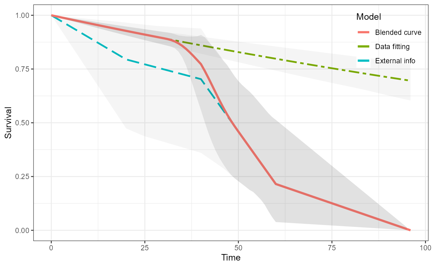
#> Chain 2:Lastly, we can run the blending step.
blend_interv <- list(min = 48, max = 150)
beta_params <- list(alpha = 3, beta = 3)
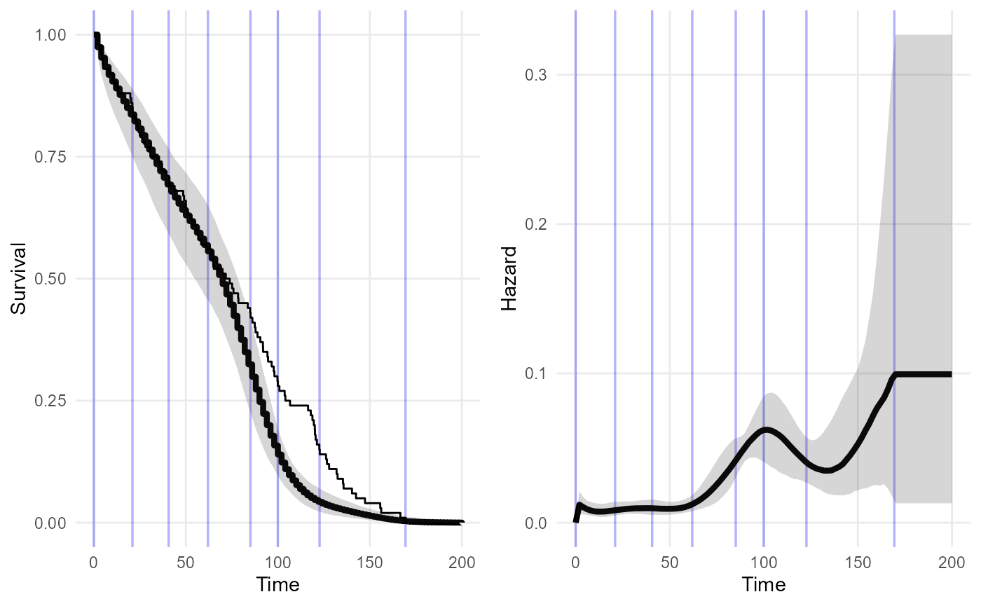
ble_Surv <- blendsurv(obs_Surv, ext_Surv, blend_interv, beta_params)
#> as(<dgCMatrix>, "dgTMatrix") is deprecated since Matrix 1.5-0; do as(., "TsparseMatrix") insteadWe can visualise all of the curves.
plot(ble_Surv)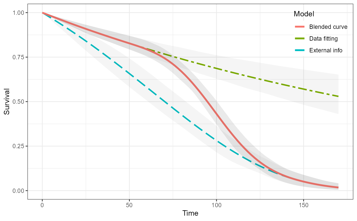
Piecewise uniform CDF
In the example above we sample from separate uniform distributions in between the times specified by the user. These data are then used to fit a parametric survival curve which is use in the blending step.
As an alternative - rather than fitting to sampled data - we could simply use the underlying survival curve directly i.e. the ‘curve’ consisting of uniform segments.
We provide the function pw_unif_surv() to create a
single piecewise uniform survival curve.
p <- c(0.05, 0)
times <- c(144, 180)
surv <- pw_unif_surv(p, times, epsilon = 1)

plot(surv, type = "l")
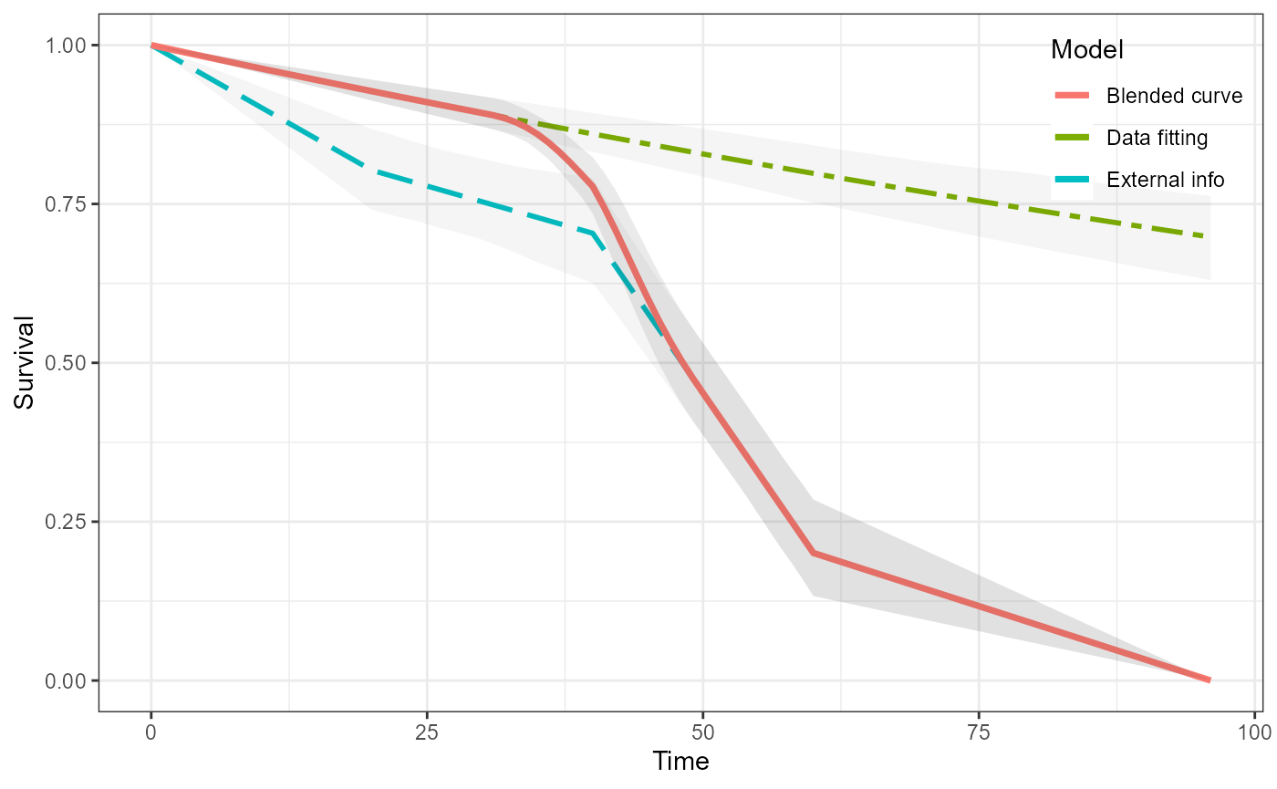
We can now simply blend the two curves together in the usual way. Because this is a single curve then there is no uncertainty associated with it.
blend_interv <- list(min = 48, max = 150)
beta_params <- list(alpha = 3, beta = 3)

ble_Surv <- blendsurv(obs_Surv, surv$S, blend_interv, beta_params)

plot(ble_Surv)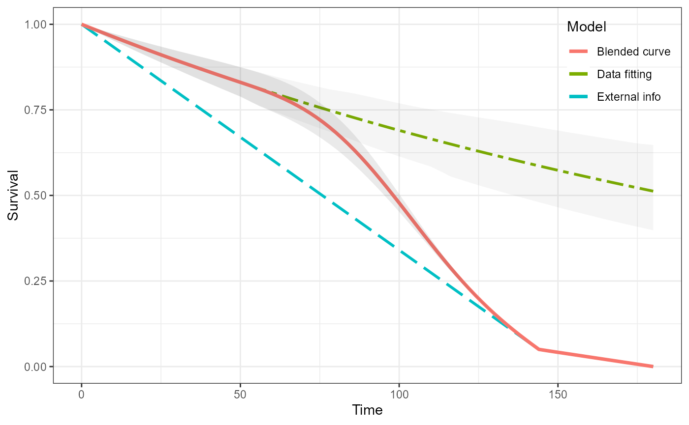
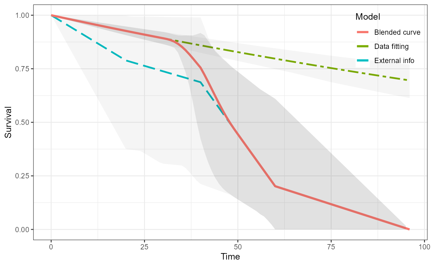
Further, one way in which we can include uncertainty on the external curve is by sampling from a Dirichlet distribution on the user-provided survival probabilities.
\[ {\bf p} \sim Dirichlet({\bf \alpha}) \]
If we use the probabilities as the parameter values of the Dirichlet distribution then the degree of certainty can be thought of as a scaling factor on these. That is for a larger scaling, i.e. taking a product with a large value, is equivalent to more certainty and vice-versa using a smaller scaling is equivalent to more uncertainty. Intuitively in a Bayesian context, we can view a hyperprior vector \(\alpha\) as pseudocounts, i.e. as representing the number of observations in each category that we have already seen.
First let us see for a moderate degree of uncertainty. We will sample
n=100 curves.
blend_interv <- list(min = 30, max = 50)
beta_params <- list(alpha = 3, beta = 3)

surv <- sample_pw_unif_surv(p = c(0.8, 0.3, 0.2, 0),
                            times = c(10, 20, 30, 48),
                            n = 100, epsilon = 0.5)

matplot(surv, type = "l")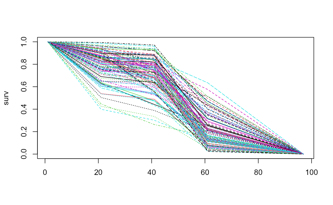
Explicitly setting the scaling factor sn=100 we can
repeat analysis this for a relatively small amount of uncertainty.
surv <- sample_pw_unif_surv(p = c(0.8, 0.3, 0.2, 0),
                            times = c(10, 20, 30, 48),
                            n = 100, epsilon = 0.5, sn = 100)

matplot(surv, type = "l")
For a large amount of uncertainty with sn=3.
surv <- sample_pw_unif_surv(p = c(0.8, 0.3, 0.2, 0),
                            times = c(10, 20, 30, 48),
                            n = 100, epsilon = 0.5, sn = 3)

matplot(surv, type = "l")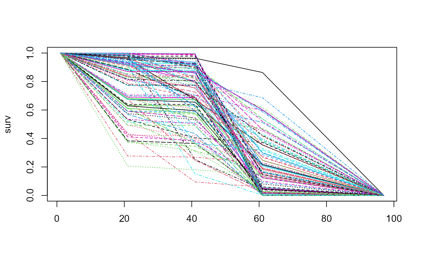
External data at landmark times as risk sets and number of events
This is related to the approach above but can be thought of as more
general. This is a format taken from Jackson and his
survextrap package (https://github.com/chjackson/survextrap/). The idea is
that at discrete pairs of time points risk set sizes and then subsequent
number of events (observed via the change in the risk set) are defined.
These can be overlapping with other risk sets and event counts. This
format allows different sizes of risk sets to be specified at different
points of time which can represent the uncertainty with the values in
the data.
blendR currently has two experimental functions for handling this
sort of input data: transform_extdata() and
riskset_surv_sim().
# transform_extdata()
# riskset_surv_sim()
# install.packages("survextrap", repos=c('https://chjackson.r-universe.dev', 'https://cloud.r-project.org'))
library(survextrap)
#> Warning: package 'survextrap' was built under R version 4.2.2
library(ggplot2)
library(dplyr)

survminer::ggsurvplot(survfit(Surv(years, status) ~ 1, data=colons), data=colons)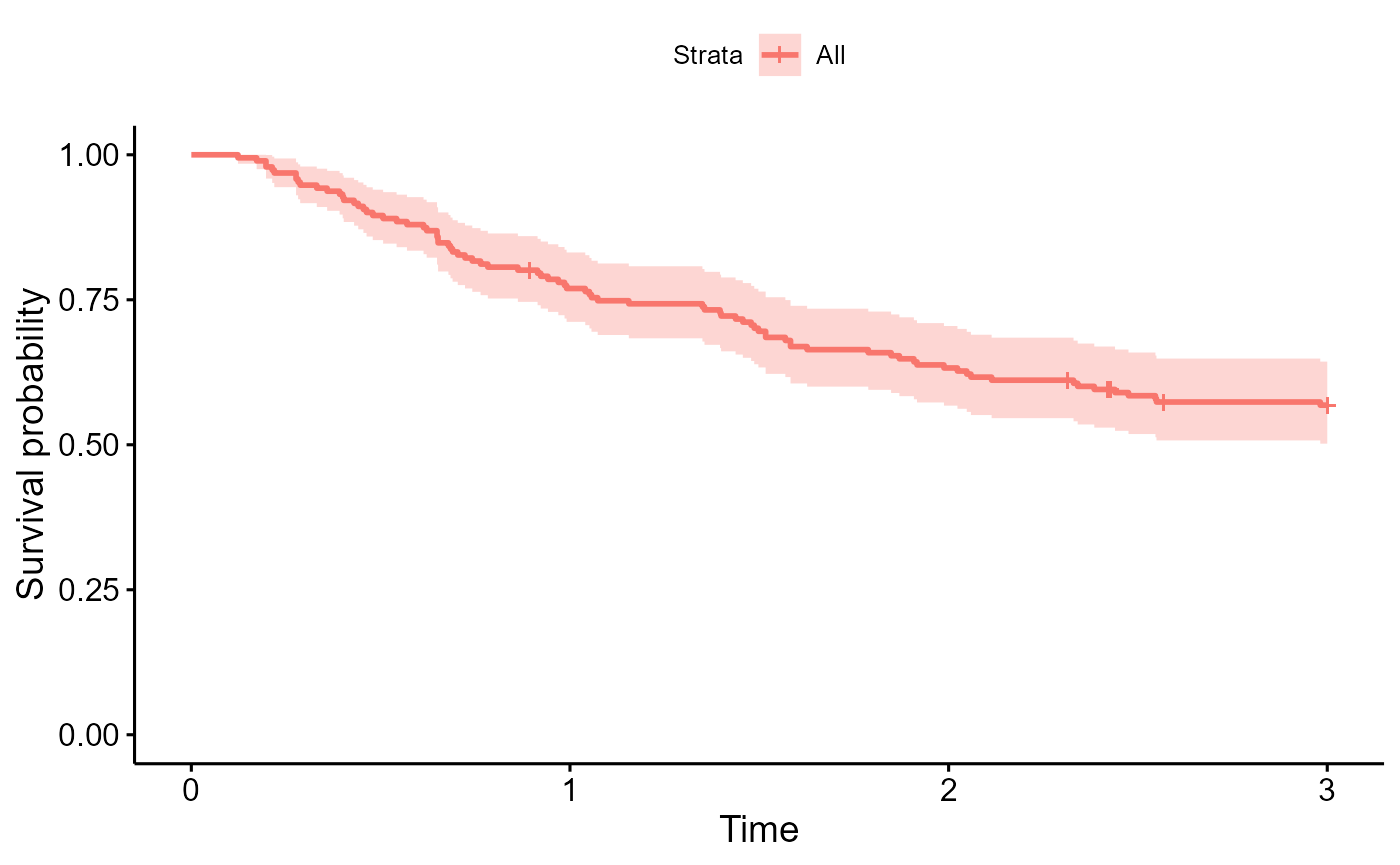
nd_mod <- survextrap(Surv(years, status) ~ 1, data=colons, chains=1)
#>
#> SAMPLING FOR MODEL 'survextrap' NOW (CHAIN 1).
#> Chain 1:
#> Chain 1: Gradient evaluation took 0 seconds
#> Chain 1: 1000 transitions using 10 leapfrog steps per transition would take 0 seconds.
#> Chain 1: Adjust your expectations accordingly!
#> Chain 1:
#> Chain 1:
#> Chain 1: Iteration:    1 / 2000 [  0%]  (Warmup)
#> Chain 1: Iteration:  200 / 2000 [ 10%]  (Warmup)
#> Chain 1: Iteration:  400 / 2000 [ 20%]  (Warmup)
#> Chain 1: Iteration:  600 / 2000 [ 30%]  (Warmup)
#> Chain 1: Iteration:  800 / 2000 [ 40%]  (Warmup)
#> Chain 1: Iteration: 1000 / 2000 [ 50%]  (Warmup)
#> Chain 1: Iteration: 1001 / 2000 [ 50%]  (Sampling)
#> Chain 1: Iteration: 1200 / 2000 [ 60%]  (Sampling)
#> Chain 1: Iteration: 1400 / 2000 [ 70%]  (Sampling)
#> Chain 1: Iteration: 1600 / 2000 [ 80%]  (Sampling)
#> Chain 1: Iteration: 1800 / 2000 [ 90%]  (Sampling)
#> Chain 1: Iteration: 2000 / 2000 [100%]  (Sampling)
#> Chain 1:
#> Chain 1:  Elapsed Time: 3.7 seconds (Warm-up)
#> Chain 1:                2.263 seconds (Sampling)
#> Chain 1:                5.963 seconds (Total)
#> Chain 1:
#> Warning: There were 2 divergent transitions after warmup. See
#> https://mc-stan.org/misc/warnings.html#divergent-transitions-after-warmup
#> to find out why this is a problem and how to eliminate them.
#> Warning: Examine the pairs() plot to diagnose sampling problems
#> Warning: Bulk Effective Samples Size (ESS) is too low, indicating posterior means and medians may be unreliable.
#> Running the chains for more iterations may help. See
#> https://mc-stan.org/misc/warnings.html#bulk-ess
#> Warning: Tail Effective Samples Size (ESS) is too low, indicating posterior variances and tail quantiles may be unreliable.
#> Running the chains for more iterations may help. See
#> https://mc-stan.org/misc/warnings.html#tail-ess
plot(nd_mod, tmax=5)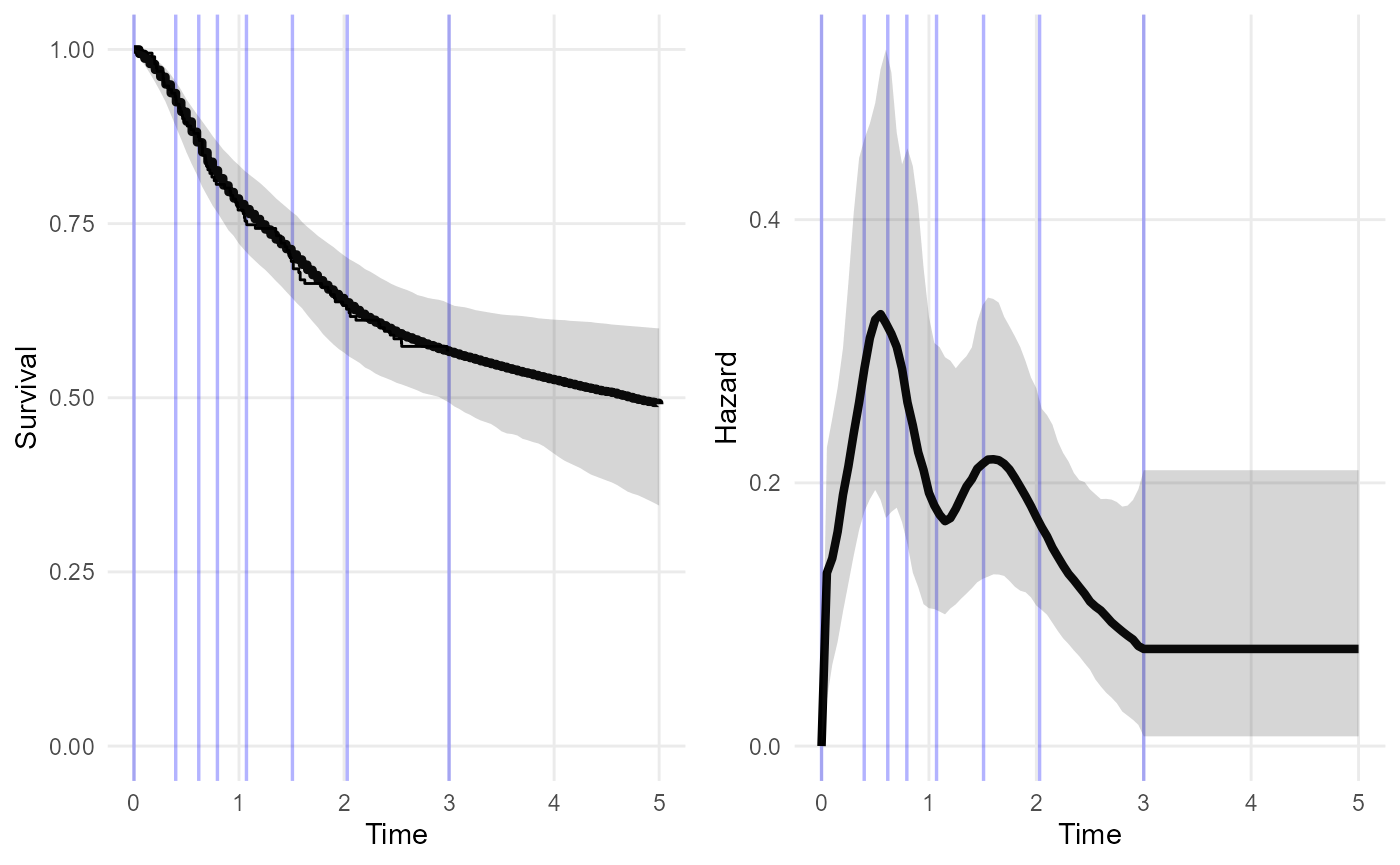
survminer::ggsurvplot(survfit(Surv(time, event) ~ 1, data=data_sim), data=data_sim)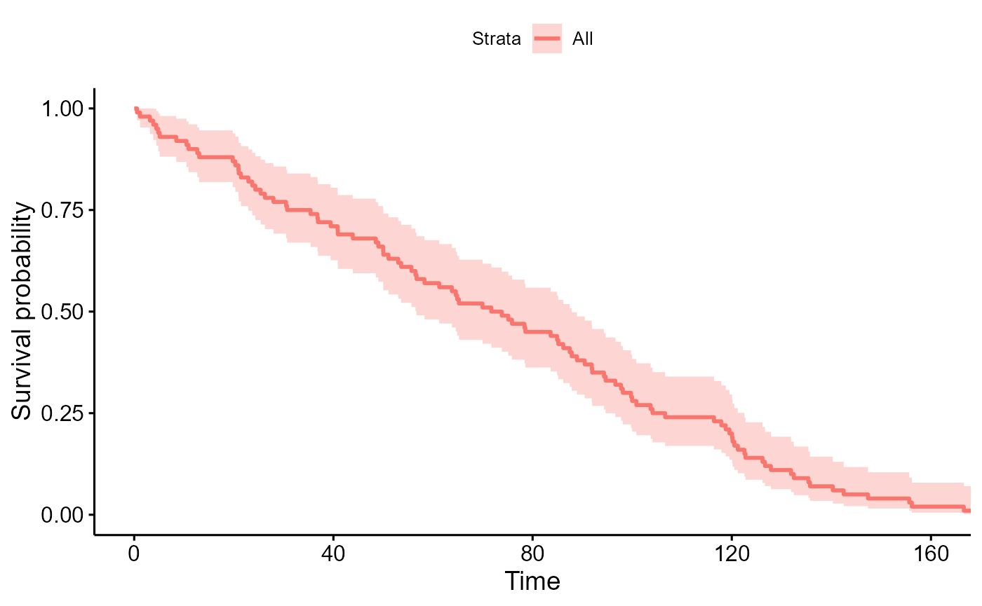
nd_mod1 <- survextrap(Surv(time, event) ~ 1, data=data_sim, chains=1)
#>
#> SAMPLING FOR MODEL 'survextrap' NOW (CHAIN 1).
#> Chain 1:
#> Chain 1: Gradient evaluation took 0.001 seconds
#> Chain 1: 1000 transitions using 10 leapfrog steps per transition would take 10 seconds.
#> Chain 1: Adjust your expectations accordingly!
#> Chain 1:
#> Chain 1:
#> Chain 1: Iteration:    1 / 2000 [  0%]  (Warmup)
#> Chain 1: Iteration:  200 / 2000 [ 10%]  (Warmup)
#> Chain 1: Iteration:  400 / 2000 [ 20%]  (Warmup)
#> Chain 1: Iteration:  600 / 2000 [ 30%]  (Warmup)
#> Chain 1: Iteration:  800 / 2000 [ 40%]  (Warmup)
#> Chain 1: Iteration: 1000 / 2000 [ 50%]  (Warmup)
#> Chain 1: Iteration: 1001 / 2000 [ 50%]  (Sampling)
#> Chain 1: Iteration: 1200 / 2000 [ 60%]  (Sampling)
#> Chain 1: Iteration: 1400 / 2000 [ 70%]  (Sampling)
#> Chain 1: Iteration: 1600 / 2000 [ 80%]  (Sampling)
#> Chain 1: Iteration: 1800 / 2000 [ 90%]  (Sampling)
#> Chain 1: Iteration: 2000 / 2000 [100%]  (Sampling)
#> Chain 1:
#> Chain 1:  Elapsed Time: 5.722 seconds (Warm-up)
#> Chain 1:                4.31 seconds (Sampling)
#> Chain 1:                10.032 seconds (Total)
#> Chain 1:
#> Warning: There were 2 divergent transitions after warmup. See
#> https://mc-stan.org/misc/warnings.html#divergent-transitions-after-warmup
#> to find out why this is a problem and how to eliminate them.
#> Warning: Examine the pairs() plot to diagnose sampling problems
#> Warning: Tail Effective Samples Size (ESS) is too low, indicating posterior variances and tail quantiles may be unreliable.
#> Running the chains for more iterations may help. See
#> https://mc-stan.org/misc/warnings.html#tail-ess
#> Warning: Some Pareto k diagnostic values are slightly high. See help('pareto-k-diagnostic') for details.
plot(nd_mod1, tmax=200)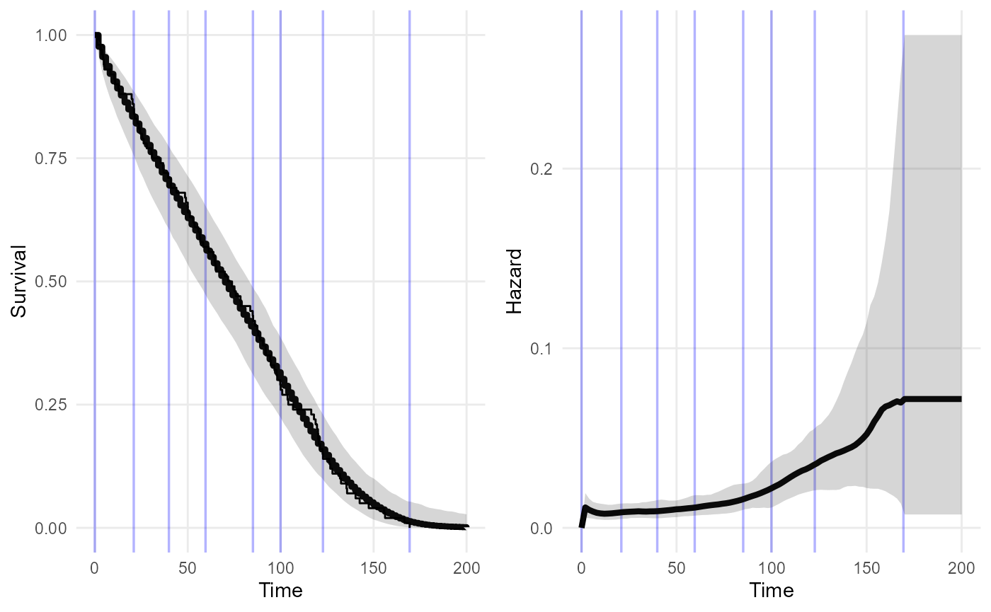
extdata <- data.frame(start = 80, stop = 100,
                      n = 100, r = 10)
nd_mod2 <- survextrap(Surv(time, event) ~ 1, data=data_sim, chains=1, external = extdata)
#>
#> SAMPLING FOR MODEL 'survextrap' NOW (CHAIN 1).
#> Chain 1:
#> Chain 1: Gradient evaluation took 0 seconds
#> Chain 1: 1000 transitions using 10 leapfrog steps per transition would take 0 seconds.
#> Chain 1: Adjust your expectations accordingly!
#> Chain 1:
#> Chain 1:
#> Chain 1: Iteration:    1 / 2000 [  0%]  (Warmup)
#> Chain 1: Iteration:  200 / 2000 [ 10%]  (Warmup)
#> Chain 1: Iteration:  400 / 2000 [ 20%]  (Warmup)
#> Chain 1: Iteration:  600 / 2000 [ 30%]  (Warmup)
#> Chain 1: Iteration:  800 / 2000 [ 40%]  (Warmup)
#> Chain 1: Iteration: 1000 / 2000 [ 50%]  (Warmup)
#> Chain 1: Iteration: 1001 / 2000 [ 50%]  (Sampling)
#> Chain 1: Iteration: 1200 / 2000 [ 60%]  (Sampling)
#> Chain 1: Iteration: 1400 / 2000 [ 70%]  (Sampling)
#> Chain 1: Iteration: 1600 / 2000 [ 80%]  (Sampling)
#> Chain 1: Iteration: 1800 / 2000 [ 90%]  (Sampling)
#> Chain 1: Iteration: 2000 / 2000 [100%]  (Sampling)
#> Chain 1:
#> Chain 1:  Elapsed Time: 4.57 seconds (Warm-up)
#> Chain 1:                3.161 seconds (Sampling)
#> Chain 1:                7.731 seconds (Total)
#> Chain 1:
plot(nd_mod2, tmax=200)