Binary data example

Introduction

This vignette will demonstrate the use of the outstandR package to fit the range of types of models to simulated binary data. Related vignettes will provide equivalent analyses for continuous and count data.

Analysis

First, let us load necessary packages.

# install.packages("outstandR",
#  repos = c("https://statisticshealtheconomics.r-universe.dev", "https://cloud.r-project.org"))
#
# install.packages("simcovariates",
#  repos = c("https://n8thangreen.r-universe.dev", "https://cloud.r-project.org"))

library(boot)      # non-parametric bootstrap in MAIC and ML G-computation
library(copula)    # simulating BC covariates from Gaussian copula
library(rstanarm)  # fit outcome regression, draw outcomes in Bayesian G-computation
library(tidyr)
library(dplyr)
library(MASS)
library(outstandR)
library(simcovariates)

Data

We consider binary outcomes using the log-odds ratio as the measure of effect. For example, the binary outcome may be response to treatment or the occurrence of an adverse event. For trials AC and BC, outcome $y_i$ for subject $i$ is simulated from a Bernoulli distribution with probabilities of success generated from logistic regression.

For the BC trial, the individual-level covariates and outcomes are aggregated to obtain summaries. The continuous covariates are summarized as means and standard deviations, which would be available to the analyst in the published study in a table of baseline characteristics in the RCT publication. The binary outcomes are summarized in an overall event table. Typically, the published study only provides aggregate information to the analyst.

The simulation input parameters are given below.

Parameter	Description	Value
`N`	Sample size	200
`allocation`	Active treatment vs. placebo allocation ratio (2:1)	2/3
`b_trt`	Conditional effect of active treatment vs. comparator (log(0.17))	-1.77196
`b_X`	Conditional effect of each prognostic variable (-log(0.5))	0.69315
`b_EM`	Conditional interaction effect of each effect modifier (-log(0.67))	0.40048
`meanX_AC[1]`	Mean of prognostic factor in AC trial	0.45
`meanX_AC[2]`	Mean of prognostic factor in AC trial	0.45
`meanX_EM_AC[1]`	Mean of effect modifier in AC trial	0.45
`meanX_EM_AC[2]`	Mean of effect modifier in AC trial	0.45
`meanX_BC[1]`	Mean of prognostic factor in BC trial	0.6
`meanX_BC[2]`	Mean of prognostic factor in BC trial	0.6
`meanX_EM_BC[1]`	Mean of effect modifier in BC trial	0.6
`meanX_EM_BC[2]`	Mean of effect modifier in BC trial	0.6
`sdX`	Standard deviation of prognostic factors (AC and BC)	0.4
`sdX_EM`	Standard deviation of effect modifiers	0.4
`corX`	Covariate correlation coefficient	0.2
`b_0`	Baseline intercept	-0.6

We shall use the gen_data() function available with the simcovariates package on GitHub.

N <- 200
allocation <- 2/3      # active treatment vs. placebo allocation ratio (2:1)
b_trt <- log(0.17)     # conditional effect of active treatment vs. common comparator
b_X <- -log(0.5)       # conditional effect of each prognostic variable
b_EM <- -log(0.67)     # conditional interaction effect of each effect modifier
meanX_AC <- c(0.45, 0.45)       # mean of normally-distributed covariate in AC trial
meanX_BC <- c(0.6, 0.6)         # mean of each normally-distributed covariate in BC
meanX_EM_AC <- c(0.45, 0.45)    # mean of normally-distributed EM covariate in AC trial
meanX_EM_BC <- c(0.6, 0.6)      # mean of each normally-distributed EM covariate in BC
sdX <- c(0.4, 0.4)     # standard deviation of each covariate (same for AC and BC)
sdX_EM <- c(0.4, 0.4)  # standard deviation of each EM covariate
corX <- 0.2            # covariate correlation coefficient  
b_0 <- -0.6            # baseline intercept coefficient  ##TODO: fixed value

covariate_defns_ipd <- list(
  PF_cont_1 = list(type = continuous(mean = meanX_AC[1], sd = sdX[1]),
                    role = "prognostic"),
  PF_cont_2 = list(type = continuous(mean = meanX_AC[2], sd = sdX[2]),
                    role = "prognostic"),
  EM_cont_1 = list(type = continuous(mean = meanX_EM_AC[1], sd = sdX_EM[1]),
                    role = "effect_modifier"),
  EM_cont_2 = list(type = continuous(mean = meanX_EM_AC[2], sd = sdX_EM[2]),
                    role = "effect_modifier")
)

b_prognostic <- c(PF_cont_1 = b_X, PF_cont_2 = b_X)

b_effect_modifier <- c(EM_cont_1 = b_EM, EM_cont_2 = b_EM)

num_normal_covs <- length(covariate_defns_ipd)
cor_matrix <- matrix(corX, num_normal_covs, num_normal_covs)
diag(cor_matrix) <- 1

rownames(cor_matrix) <- c("PF_cont_1", "PF_cont_2", "EM_cont_1", "EM_cont_2")
colnames(cor_matrix) <- c("PF_cont_1", "PF_cont_2", "EM_cont_1", "EM_cont_2")

ipd_trial <- simcovariates::gen_data(
  N = N,
  b_0 = b_0,
  b_trt = b_trt,
  covariate_defns = covariate_defns_ipd,
  b_prognostic = b_prognostic,
  b_effect_modifier = b_effect_modifier,
  cor_matrix = cor_matrix,
  trt_assignment = list(prob_trt1 = allocation),
  family = binomial("logit"))

The treatment column in the return data is binary and takes values 0 and 1. We will include some extra information about treatment names. To do this we will define the lable of the two level factor as A for 1 and C for 0 as follows.

ipd_trial$trt <- factor(ipd_trial$trt, labels = c("C", "A"))

Similarly, to obtain the aggregate data we will simulate IPD but with the additional summarise step. We set different mean values meanX_BC and meanX_EM_BC but otherwise use the same parameter values as for the $AC$ trial.

covariate_defns_ald <- list(
  PF_cont_1 = list(type = continuous(mean = meanX_BC[1], sd = sdX[1]),
                    role = "prognostic"),
  PF_cont_2 = list(type = continuous(mean = meanX_BC[2], sd = sdX[2]),
                    role = "prognostic"),
  EM_cont_1 = list(type = continuous(mean = meanX_EM_BC[1], sd = sdX_EM[1]),
                    role = "effect_modifier"),
  EM_cont_2 = list(type = continuous(mean = meanX_EM_BC[2], sd = sdX_EM[2]),
                    role = "effect_modifier")
)

BC.IPD <- simcovariates::gen_data(
  N = N,
  b_0 = b_0,
  b_trt = b_trt,
  covariate_defns = covariate_defns_ald,
  b_prognostic = b_prognostic,
  b_effect_modifier = b_effect_modifier,
  cor_matrix = cor_matrix,
  trt_assignment = list(prob_trt1 = allocation),
  family = binomial("logit"))

BC.IPD$trt <- factor(BC.IPD$trt, labels = c("C", "B"))

# covariate summary statistics
# assume same between treatments
cov.X <- 
  BC.IPD %>%
  as.data.frame() |> 
  dplyr::select(matches("^(PF|EM)"), trt) |> 
  tidyr::pivot_longer(
    cols = starts_with("PF") | starts_with("EM"),
    names_to = "variable",
    values_to = "value") |>
  group_by(variable) %>%
  summarise(
    mean = mean(value),
    sd = sd(value)
  ) %>%
  tidyr::pivot_longer(
    cols = c("mean", "sd"),
    names_to = "statistic",
    values_to = "value") %>%
  ungroup() |> 
  mutate(trt = NA)

# outcome
summary.y <- 
  BC.IPD |> 
  as.data.frame() |> 
  dplyr::select(y, trt) %>%
  tidyr::pivot_longer(cols = "y",
               names_to = "variable",
               values_to = "value") %>%
  group_by(variable, trt) %>%
  summarise(
    mean = mean(value),
    sd = sd(value),
    sum = sum(value)
  ) %>%
  tidyr::pivot_longer(
    cols = c("mean", "sd", "sum"),
    names_to = "statistic",
    values_to = "value") %>%
  ungroup()
#> `summarise()` has grouped output by 'variable'. You can override using the
#> `.groups` argument.

# sample sizes
summary.N <- 
  BC.IPD |> 
  group_by(trt) |> 
  count(name = "N") |> 
  tidyr::pivot_longer(
    cols = "N",
    names_to = "statistic",
    values_to = "value") |> 
  mutate(variable = NA_character_) |> 
  dplyr::select(variable, statistic, value, trt)
  
ald_trial <- rbind.data.frame(cov.X, summary.y, summary.N)

This general format of the data sets are in a ‘long’ style consisting of the following.

`ipd_trial`: Individual patient data

PF_*: Patient measurements prognostic factors
EM_*: Patient measurements effect modifiers
trt: Treatment label (factor)
y: Indicator of whether event was observed (two level factor)

`ald_trial`: Aggregate-level data

variable: Covariate name. In the case of treatment arm sample size this is NA
statistic: Summary statistic name from mean, standard deviation or sum
value: Numerical value of summary statistic
trt: Treatment label. Because we assume a common covariate distribution between treatment arms this is NA

Our data look like the following.

head(ipd_trial)
#>   id   PF_cont_1   PF_cont_2  EM_cont_1   EM_cont_2 trt y     true_eta
#> 1  1  0.75056436  0.95597583  0.3158969  1.19430733   C 0  0.582883524
#> 2  2  0.83246940  0.11789773  0.5094678  0.08180243   A 1 -1.476422106
#> 3  3  1.13401333  1.15036919  1.2342379  0.74771694   A 0  0.005184912
#> 4  4  0.78518298  0.83080451 -0.1625820  0.35223227   C 1  0.520117172
#> 5  5 -0.38547667  0.87070020  0.7213797 -0.03557032   A 1 -1.760974264
#> 6  6 -0.04851591 -0.03013213  0.6580067  0.05853054   A 0 -2.139514435

There are 4 correlated continuous covariates generated per subject, simulated from a multivariate normal distribution. Treatment trt takes either new treatment A or standard of care / status quo C. The ITC is ‘anchored’ via C, the common treatment.

ald_trial
#> # A tibble: 16 × 4
#>    variable  statistic   value trt  
#>    <chr>     <chr>       <dbl> <chr>
#>  1 EM_cont_1 mean        0.616 NA   
#>  2 EM_cont_1 sd          0.408 NA   
#>  3 EM_cont_2 mean        0.635 NA   
#>  4 EM_cont_2 sd          0.354 NA   
#>  5 PF_cont_1 mean        0.666 NA   
#>  6 PF_cont_1 sd          0.398 NA   
#>  7 PF_cont_2 mean        0.663 NA   
#>  8 PF_cont_2 sd          0.404 NA   
#>  9 y         mean        0.597 C    
#> 10 y         sd          0.494 C    
#> 11 y         sum        43     C    
#> 12 y         mean        0.297 B    
#> 13 y         sd          0.459 B    
#> 14 y         sum        38     B    
#> 15 NA        N          72     C    
#> 16 NA        N         128     B

In this case, we have 4 covariate mean and standard deviation values; and the event total, average and sample size for each treatment B and C.

Regression model

The true logistic outcome model which we use to simulate the data is

$\text{logit}(p_{t}) = \beta_0 + \beta_X (X_3 + X_4) + [\beta_{t} + \beta_{EM} (X_1 + X_2)] \; \text{I}(t \neq C)$

$\text{I}()$ is an indicator function taking value 1 if true and 0 otherwise. That is, for treatment $C$ the right hand side becomes $\beta_0 + \beta_X (X_3 + X_4)$ and for comparator treatments $A$ or $B$ there is an additional $\beta_t + \beta_{EM} (X_1 + X_2)$ component consisting of the effect modifier terms and the coefficient for the treatment parameter, $\beta_t$ (or b_trt in the R code), i.e. the log odds-ratio (LOR) for the logit model. Finally, $p_{t}$ is the probability of experiencing the event of interest for treatment $t$ .

Output statistics

We will obtain the marginal treatment effect and marginal variance. The definition by which of these are calculated depends on the type of data and outcome scale. For our current example of binary data and log-odds ratio the marginal treatment effect is

$\log\left( \frac{n_B/(N_B-n_B)}{n_C/(N_B-n_{B})} \right) = \log(n_B n_{\bar{C}}) - \log(n_C n_{\bar{B}})$

and marginal variance is

$\frac{1}{n_C} + \frac{1}{n_{\bar{C}}} + \frac{1}{n_B} + \frac{1}{n_{\bar{B}}}$

where $n_B, n_C$ are the number of events in each arm and $\bar{C}$ is the compliment of $C$ , so e.g. $n_{\bar{C}} = N_C - n_c$ . Other outcome scales will be discussed below.

Model fitting in R

The outstandR package has been written to be easy to use and essentially consists of a single function, outstandR(). This can be used to run all of the different types of model, which when combined with their specific parameters we will call strategies. The first two arguments of outstandR() are the individual patient and aggregate-level data, respectively.

A strategy argument of outstandR takes functions called strategy_*(), where the wildcard * is replaced by the name of the particular method required, e.g. strategy_maic() for MAIC. Each specific example is provided below.

Model formula

We will take advantage of the in-built R formula object to define the models. This will allow us to easily pull out components of the object and consistently use it. Defining $EM\_cont\_1, EM\_cont\_2$ as effect modifiers, $PF\_cont\_1, PF\_cont\_2$ as prognostic variables and $Z$ the treatment indicator then the formula used in this model is

$y = PF\_cont\_1 + PF\_cont\_2 + Z + Z \times EM\_cont\_1 + Z \times EM\_cont\_2$

Notice that this does not include the link function of interest so appears as a linear regression. This corresponds to the following R formula object we will pass as an argument to the strategy function.

lin_form <- as.formula("y ~ PF_cont_1 + PF_cont_2 + trt + trt:EM_cont_1 + trt:EM_cont_2")

Note that the more succinct formula

y ~ PF_cont_1 + PF_cont_2 + trt*(EM_cont_1 + EM_cont_2)

would additionally include $X_1, X_2$ as prognostic factors so is not equivalent (but this may be what you actually want). To recover the original formula it can be modified as follows.

y ~ PF_cont_1 + PF_cont_2 + trt*(EM_cont_1 + EM_cont_2) - EM_cont_1 - EM_cont_2

We note that the MAIC approach does not strictly use a regression in the same way as the other methods so should not be considered directly comparable in this sense but we have decided to use a consistent syntax across models using ‘formula’.

Matching-Adjusted Indirect Comparison (MAIC)

A single call to outstandR() is sufficient to run the model. We pass to the strategy argument the strategy_maic() function with arguments formula = lin_form as defined above and family = binomial(link = "logit") for binary data and logistic link.

Internally, using the individual patient level data for AC firstly we perform non-parametric bootstrap of the maic.boot function with R = 1000 replicates. This function fits treatment coefficient for the marginal effect for A vs C. The returned value is an object of class boot from the {boot} package. We then calculate the bootstrap mean and variance in the wrapper function maic_boot_stats.

outstandR_maic <-
  outstandR(ipd_trial, ald_trial,
            strategy = strategy_maic(
              formula = lin_form,
              family = binomial(link = "logit")))

The returned object is of class outstandR.

str(outstandR_maic)
#> List of 2
#>  $ contrasts:List of 3
#>   ..$ means    :List of 3
#>   .. ..$ AB: num 0.607
#>   .. ..$ AC: num -0.649
#>   .. ..$ BC: num -1.26
#>   ..$ variances:List of 3
#>   .. ..$ AB: num 0.233
#>   .. ..$ AC: num 0.137
#>   .. ..$ BC: num 0.0952
#>   ..$ CI       :List of 3
#>   .. ..$ AB: num [1:2] -0.338 1.552
#>   .. ..$ AC: num [1:2] -1.3757 0.0776
#>   .. ..$ BC: num [1:2] -1.861 -0.652
#>  $ absolute :List of 2
#>   ..$ means    :List of 2
#>   .. ..$ A: Named num 0.341
#>   .. .. ..- attr(*, "names")= chr "mean_A"
#>   .. ..$ C: Named num 0.495
#>   .. .. ..- attr(*, "names")= chr "mean_C"
#>   ..$ variances:List of 2
#>   .. ..$ A: Named num 0.00271
#>   .. .. ..- attr(*, "names")= chr "mean_A"
#>   .. ..$ C: Named num 0.00518
#>   .. .. ..- attr(*, "names")= chr "mean_C"
#>  - attr(*, "CI")= num 0.95
#>  - attr(*, "ref_trt")= chr "C"
#>  - attr(*, "scale")= chr "log_odds"
#>  - attr(*, "model")= chr "binomial"
#>  - attr(*, "class")= chr [1:2] "outstandR" "list"

We see that this is a list object with 2 parts. The first contains statistics between each pair of treatments. These are the mean contrasts, variances and confidence intervals (CI), respectively. The default CI is for 95% but can be altered in outstandR with the CI argument. The second element of the list contains the absolute effect estimates.

A print method is available for outstandR objects for more human-readable output

outstandR_maic
#> Object of class 'outstandR' 
#> Model: binomial 
#> Scale: log_odds 
#> Common treatment: C 
#> Individual patient data study: AC 
#> Aggregate level data study: BC 
#> Confidence interval level: 0.95 
#> 
#> Contrasts:
#> 
#> # A tibble: 3 × 5
#>   Treatments Estimate Std.Error lower.0.95 upper.0.95
#>   <chr>         <dbl>     <dbl>      <dbl>      <dbl>
#> 1 AB            0.607    0.233      -0.338     1.55  
#> 2 AC           -0.649    0.137      -1.38      0.0776
#> 3 BC           -1.26     0.0952     -1.86     -0.652 
#> 
#> Absolute:
#> 
#> # A tibble: 2 × 5
#>   Treatments Estimate Std.Error lower.0.95 upper.0.95
#>   <chr>         <dbl>     <dbl> <lgl>      <lgl>     
#> 1 A             0.341   0.00271 NA         NA        
#> 2 C             0.495   0.00518 NA         NA

Outcome scale

If we do not explicitly specify the outcome scale, the default is that used to fit to the data in the regression model. As we saw, in this case, the default is log-odds ratio corresponding to the "logit" link function for binary data. However, we can change this to some other scale which may be more appropriate for a particular analysis. So far implemented in the package, the links and their corresponding relative treatment effect scales are as follows:

Data Type	Model	Scale	Argument
Binary	`logit`	Log-odds ratio	`log_odds`
Count	`log`	Log-risk ratio	`log_relative_risk`
Continuous	`mean`	Mean difference	`risk_difference`

The full list of possible transformed treatment effect scales will be: log-odds ratio, log-risk ratio, mean difference, risk difference, hazard ratio, hazard difference.

For binary data the marginal treatment effect and variance are

Log-risk ratio

Treatment effect is

$\log(n_B/N_B) - \log(n_A/N_A)$

and variance

$\frac{1}{n_B} - \frac{1}{N_B} + \frac{1}{n_A} - \frac{1}{N_A}$

Risk difference

Treatment effect is

$\frac{n_B}{N_B} - \frac{n_A}{N_A}$

and variance

$\frac{n_B}{N_B} \left( 1 - \frac{n_B}{N_B} \right) + \frac{n_A}{N_A} \left( 1 - \frac{n_A}{N_A} \right)$

To change the outcome scale, we can pass the scale argument in the outstandR() function. For example, to change the scale to risk difference, we can use the following code.

outstandR_maic_lrr <-
  outstandR(ipd_trial, ald_trial,
            strategy = strategy_maic(formula = lin_form,
                                     family = binomial(link = "logit")),
            scale = "log_relative_risk")

outstandR_maic_lrr
#> Object of class 'outstandR' 
#> Model: binomial 
#> Scale: log_relative_risk 
#> Common treatment: C 
#> Individual patient data study: AC 
#> Aggregate level data study: BC 
#> Confidence interval level: 0.95 
#> 
#> Contrasts:
#> 
#> # A tibble: 3 × 5
#>   Treatments Estimate Std.Error lower.0.95 upper.0.95
#>   <chr>         <dbl>     <dbl>      <dbl>      <dbl>
#> 1 AB            0.307    0.0793     -0.244     0.859 
#> 2 AC           -0.392    0.0514     -0.836     0.0527
#> 3 BC           -0.699    0.0279     -1.03     -0.372 
#> 
#> Absolute:
#> 
#> # A tibble: 2 × 5
#>   Treatments Estimate Std.Error lower.0.95 upper.0.95
#>   <chr>         <dbl>     <dbl> <lgl>      <lgl>     
#> 1 A             0.339   0.00258 NA         NA        
#> 2 C             0.501   0.00537 NA         NA

Simulated treatment comparison (STC)

Simulated treatment comparison (STC) is the conventional outcome regression method. It involves fitting a regression model of outcome on treatment and covariates to the IPD anad then ‘plugging-in’ mean covariate values from the aggregate data study.

We can simply pass the same formula as before to the modified call with strategy_stc().

outstandR_stc <-
  outstandR(ipd_trial, ald_trial,
            strategy = strategy_stc(
              formula = lin_form,
              family = binomial(link = "logit")))

outstandR_stc
#> Object of class 'outstandR' 
#> Model: binomial 
#> Scale: log_odds 
#> Common treatment: C 
#> Individual patient data study: AC 
#> Aggregate level data study: BC 
#> Confidence interval level: 0.95 
#> 
#> Contrasts:
#> 
#> # A tibble: 3 × 5
#>   Treatments Estimate Std.Error lower.0.95 upper.0.95
#>   <chr>         <dbl>     <dbl>      <dbl>      <dbl>
#> 1 AB           0.0584   NA           NA        NA    
#> 2 AC          -1.20     NA           NA        NA    
#> 3 BC          -1.26      0.0952      -1.86     -0.652
#> 
#> Absolute:
#> 
#> # A tibble: 2 × 5
#>   Treatments Estimate Std.Error lower.0.95 upper.0.95
#>   <chr>         <dbl>     <dbl> <lgl>      <lgl>     
#> 1 A             0.137        NA NA         NA        
#> 2 C             0.344        NA NA         NA

Changing the outcome scale to LRR gives

outstandR_stc_lrr <-
  outstandR(ipd_trial, ald_trial,
            strategy = strategy_stc(
              formula = lin_form,
              family = binomial(link = "logit")),
            scale = "log_relative_risk")

outstandR_stc_lrr
#> Object of class 'outstandR' 
#> Model: binomial 
#> Scale: log_relative_risk 
#> Common treatment: C 
#> Individual patient data study: AC 
#> Aggregate level data study: BC 
#> Confidence interval level: 0.95 
#> 
#> Contrasts:
#> 
#> # A tibble: 3 × 5
#>   Treatments Estimate Std.Error lower.0.95 upper.0.95
#>   <chr>         <dbl>     <dbl>      <dbl>      <dbl>
#> 1 AB           -0.224   NA           NA        NA    
#> 2 AC           -0.923   NA           NA        NA    
#> 3 BC           -0.699    0.0279      -1.03     -0.372
#> 
#> Absolute:
#> 
#> # A tibble: 2 × 5
#>   Treatments Estimate Std.Error lower.0.95 upper.0.95
#>   <chr>         <dbl>     <dbl> <lgl>      <lgl>     
#> 1 A             0.137        NA NA         NA        
#> 2 C             0.344        NA NA         NA

The following approaches follow naturally from the simple ‘plug-in’ version of STC. We will perform G-computation firstly with a frequentist MLE and then a Bayesian approach.

Parametric G-computation with maximum-likelihood estimation

G-computation marginalizes the conditional estimates by separating the regression modelling from the estimation of the marginal treatment effect for A versus C. First, a regression model of the observed outcome $y$ on the covariates $x$ and treatment $z$ is fitted to the AC IPD:

$g(\mu_n) = \beta_0 + \boldsymbol{x}_n \boldsymbol{\beta_X} + (\beta_z + \boldsymbol{x_n^{EM}} \boldsymbol{\beta_{EM}}) \; \mbox{I}(t \neq C)$

In the context of G-computation, this regression model is often called the “Q-model.” Having fitted the Q-model, the regression coefficients are treated as nuisance parameters. The parameters are applied to the simulated covariates $x*$ to predict hypothetical outcomes for each subject under both possible treatments. Namely, a pair of predicted outcomes, also called potential outcomes, under A and under C, is generated for each subject.

By plugging treatment C into the regression fit for every simulated observation, we predict the marginal outcome mean in the hypothetical scenario in which all units are under treatment C:

$\hat{\mu}_0 = \int_{x^*} g^{-1} (\hat{\beta}_0 + x^* \hat{\beta}_1 ) p(x^*) \; \text{d}x^*$

As performed for the previous approaches, call outstandR() but change the strategy to strategy_gcomp_ml(),

outstandR_gcomp_ml <-
  outstandR(ipd_trial, ald_trial,
            strategy = strategy_gcomp_ml(
              formula = lin_form,
              family = binomial(link = "logit")))

outstandR_gcomp_ml
#> Object of class 'outstandR' 
#> Model: binomial 
#> Scale: log_odds 
#> Common treatment: C 
#> Individual patient data study: AC 
#> Aggregate level data study: BC 
#> Confidence interval level: 0.95 
#> 
#> Contrasts:
#> 
#> # A tibble: 3 × 5
#>   Treatments Estimate Std.Error lower.0.95 upper.0.95
#>   <chr>         <dbl>     <dbl>      <dbl>      <dbl>
#> 1 AB            0.602    0.232      -0.342     1.55  
#> 2 AC           -0.654    0.137      -1.38      0.0714
#> 3 BC           -1.26     0.0952     -1.86     -0.652 
#> 
#> Absolute:
#> 
#> # A tibble: 2 × 5
#>   Treatments Estimate Std.Error lower.0.95 upper.0.95
#>   <chr>         <dbl>     <dbl> <lgl>      <lgl>     
#> 1 A             0.411   0.00291 NA         NA        
#> 2 C             0.570   0.00563 NA         NA

Once again, let us change the outcome scale to LRR

outstandR_gcomp_ml_lrr <-
  outstandR(ipd_trial, ald_trial,
            strategy = strategy_gcomp_ml(
              formula = lin_form,
              family = binomial(link = "logit")),
            scale = "log_relative_risk")

outstandR_gcomp_ml_lrr
#> Object of class 'outstandR' 
#> Model: binomial 
#> Scale: log_relative_risk 
#> Common treatment: C 
#> Individual patient data study: AC 
#> Aggregate level data study: BC 
#> Confidence interval level: 0.95 
#> 
#> Contrasts:
#> 
#> # A tibble: 3 × 5
#>   Treatments Estimate Std.Error lower.0.95 upper.0.95
#>   <chr>         <dbl>     <dbl>      <dbl>      <dbl>
#> 1 AB            0.377    0.0602     -0.104     0.858 
#> 2 AC           -0.322    0.0323     -0.674     0.0307
#> 3 BC           -0.699    0.0279     -1.03     -0.372 
#> 
#> Absolute:
#> 
#> # A tibble: 2 × 5
#>   Treatments Estimate Std.Error lower.0.95 upper.0.95
#>   <chr>         <dbl>     <dbl> <lgl>      <lgl>     
#> 1 A             0.409   0.00276 NA         NA        
#> 2 C             0.563   0.00504 NA         NA

Bayesian G-computation with MCMC

The difference between Bayesian G-computation and its maximum-likelihood counterpart is in the estimated distribution of the predicted outcomes. The Bayesian approach also marginalizes, integrates or standardizes over the joint posterior distribution of the conditional nuisance parameters of the outcome regression, as well as the joint covariate distribution.

Draw a vector of size $N^*$ of predicted outcomes $y^*_z$ under each set intervention $z^* \in \{0, 1\}$ from its posterior predictive distribution under the specific treatment. This is defined as $p(y^*_{z^*} \mid \mathcal{D}_{AC}) = \int_{\beta} p(y^*_{z^*} \mid \beta) p(\beta \mid \mathcal{D}_{AC}) d\beta$ where $p(\beta \mid \mathcal{D}_{AC})$ is the posterior distribution of the outcome regression coefficients $\beta$ , which encode the predictor-outcome relationships observed in the AC trial IPD. This is given by:

$p(y^*_{^z*} \mid \mathcal{D}_{AC}) = \int_{x^*} p(y^* \mid z^*, x^*, \mathcal{D}_{AC}) p(x^* \mid \mathcal{D}_{AC})\; \text{d}x^*$

$= \int_{x^*} \int_{\beta} p(y^* \mid z^*, x^*, \beta) p(x^* \mid \beta) p(\beta \mid \mathcal{D}_{AC})\; d\beta \; \text{d}x^*$

In practice, the integrals above can be approximated numerically, using full Bayesian estimation via Markov chain Monte Carlo (MCMC) sampling.

The average, variance and interval estimates of the marginal treatment effect can be derived empirically from draws of the posterior density.

The strategy function to plug-in to the outstandR() call for this approach is strategy_gcomp_stan(),

outstandR_gcomp_stan <-
  outstandR(ipd_trial, ald_trial,
            strategy = strategy_gcomp_stan(
              formula = lin_form,
              family = binomial(link = "logit")))

outstandR_gcomp_stan
#> Object of class 'outstandR' 
#> Model: binomial 
#> Scale: log_odds 
#> Common treatment: C 
#> Individual patient data study: AC 
#> Aggregate level data study: BC 
#> Confidence interval level: 0.95 
#> 
#> Contrasts:
#> 
#> # A tibble: 3 × 5
#>   Treatments Estimate Std.Error lower.0.95 upper.0.95
#>   <chr>         <dbl>     <dbl>      <dbl>      <dbl>
#> 1 AB            0.612    0.228      -0.325     1.55  
#> 2 AC           -0.644    0.133      -1.36      0.0713
#> 3 BC           -1.26     0.0952     -1.86     -0.652 
#> 
#> Absolute:
#> 
#> # A tibble: 2 × 5
#>   Treatments Estimate Std.Error lower.0.95 upper.0.95
#>   <chr>         <dbl>     <dbl> <lgl>      <lgl>     
#> 1 A             0.411   0.00288 NA         NA        
#> 2 C             0.568   0.00521 NA         NA

As before, we can change the outcome scale to LRR.

outstandR_gcomp_stan_lrr <-
  outstandR(ipd_trial, ald_trial,
            strategy = strategy_gcomp_stan(
              formula = lin_form,
              family = binomial(link = "logit")),
            scale = "log_relative_risk")

outstandR_gcomp_stan_lrr
#> Object of class 'outstandR' 
#> Model: binomial 
#> Scale: log_relative_risk 
#> Common treatment: C 
#> Individual patient data study: AC 
#> Aggregate level data study: BC 
#> Confidence interval level: 0.95 
#> 
#> Contrasts:
#> 
#> # A tibble: 3 × 5
#>   Treatments Estimate Std.Error lower.0.95 upper.0.95
#>   <chr>         <dbl>     <dbl>      <dbl>      <dbl>
#> 1 AB            0.375    0.0607     -0.108     0.858 
#> 2 AC           -0.324    0.0328     -0.679     0.0308
#> 3 BC           -0.699    0.0279     -1.03     -0.372 
#> 
#> Absolute:
#> 
#> # A tibble: 2 × 5
#>   Treatments Estimate Std.Error lower.0.95 upper.0.95
#>   <chr>         <dbl>     <dbl> <lgl>      <lgl>     
#> 1 A             0.411   0.00288 NA         NA        
#> 2 C             0.568   0.00521 NA         NA

Multiple imputation marginalisation

The final method is to obtain the marginalized treatment effect for aggregate level data study, obtained by integrating over the covariate distribution from the aggregate level data $BC$ study

$\Delta^{\text{marg}} = \mathbb{E}_{X \sim f_{\text{BC}}(X)} \left[ \mu_{T=1}(X) - \mu_{T=0}(X) \right] = \int \left[ \mu_{T=1}(X) - \mu_{T=0}(X) \right] f_{\text{BC}}(X) \; \text{d}X$

The aggregate level data likelihood is

$\hat{\Delta}_{BC} \sim \mathcal{N}(\Delta^{\text{marg}}, SE^2)$

The multiple imputation marginalisation strategy function is strategy_mim(),

outstandR_mim <-
  outstandR(ipd_trial, ald_trial,
            strategy = strategy_mim(
              formula = lin_form,
              family = binomial(link = "logit")))

outstandR_mim
#> Object of class 'outstandR' 
#> Model: binomial 
#> Scale: log_odds 
#> Common treatment: C 
#> Individual patient data study: AC 
#> Aggregate level data study: BC 
#> Confidence interval level: 0.95 
#> 
#> Contrasts:
#> 
#> # A tibble: 3 × 5
#>   Treatments Estimate Std.Error lower.0.95 upper.0.95
#>   <chr>         <dbl>     <dbl>      <dbl>      <dbl>
#> 1 AB            0.612    0.216      -0.299     1.52  
#> 2 AC           -0.644    0.121      -1.33      0.0386
#> 3 BC           -1.26     0.0952     -1.86     -0.652 
#> 
#> Absolute:
#> 
#> # A tibble: 2 × 5
#>   Treatments Estimate Std.Error lower.0.95 upper.0.95
#>   <chr>      <lgl>    <lgl>     <lgl>      <lgl>     
#> 1 A          NA       NA        NA         NA        
#> 2 C          NA       NA        NA         NA

Change the outcome scale again for LRR,

outstandR_mim_lrr <-
  outstandR(ipd_trial, ald_trial,
            strategy = strategy_mim(
              formula = lin_form,
              family = binomial(link = "logit")),
            scale = "log_relative_risk")

outstandR_mim_lrr
#> Object of class 'outstandR' 
#> Model: binomial 
#> Scale: log_relative_risk 
#> Common treatment: C 
#> Individual patient data study: AC 
#> Aggregate level data study: BC 
#> Confidence interval level: 0.95 
#> 
#> Contrasts:
#> 
#> # A tibble: 3 × 5
#>   Treatments Estimate Std.Error lower.0.95 upper.0.95
#>   <chr>         <dbl>     <dbl>      <dbl>      <dbl>
#> 1 AB            0.375    0.0516    -0.0704     0.820 
#> 2 AC           -0.324    0.0237    -0.626     -0.0227
#> 3 BC           -0.699    0.0279    -1.03      -0.372 
#> 
#> Absolute:
#> 
#> # A tibble: 2 × 5
#>   Treatments Estimate Std.Error lower.0.95 upper.0.95
#>   <chr>      <lgl>    <lgl>     <lgl>      <lgl>     
#> 1 A          NA       NA        NA         NA        
#> 2 C          NA       NA        NA         NA

Model comparison

$AC$ effect in $BC$ population

The true $AC$ effect on the log OR scale in the $BC$ (aggregate trial data) population is $\beta_t^{AC} + \beta_{EM} (\bar{X}^{AC}_1 + \bar{X}_2^{AC})$ . Calculated by

mean_X1 <- ald_trial$value[ald_trial$statistic == "mean" & ald_trial$variable == "EM_cont_1"]
mean_X2 <- ald_trial$value[ald_trial$statistic == "mean" & ald_trial$variable == "EM_cont_1"]

d_AC_true <- b_trt + b_EM * (mean_X1 + mean_X2)

The naive approach is to just convert directly from one population to another, ignoring the imbalance in effect modifiers.

d_AC_naive <- 
  ipd_trial |> 
  dplyr::group_by(trt) |> 
  dplyr::summarise(y_sum = sum(y), y_bar = mean(y), n = n()) |> 
  tidyr::pivot_wider(names_from = trt,
                     values_from = c(y_sum, y_bar, n)) |> 
  dplyr::mutate(d_AC =
                  log(y_bar_A/(1-y_bar_A)) - log(y_bar_C/(1-y_bar_C)),
                var_AC =
                  1/(n_A-y_sum_A) + 1/y_sum_A + 1/(n_C-y_sum_C) + 1/y_sum_C)

$AB$ effect in $BC$ population

This is the indirect effect. The true $AB$ effect in the $BC$ population is $\beta_t^{AC} - \beta_t^{BC}$ .

Following the simulation study in Remiro et al (2020) these cancel out and the true effect is zero.

The naive comparison calculating $AB$ effect in the $BC$ population is

# reshape to make extraction easier
ald_out <- ald_trial |> 
  dplyr::filter(variable == "y" | is.na(variable)) |> 
  mutate(stat_trt = paste0(statistic, "_", trt)) |> 
  dplyr::select(stat_trt, value) |> 
  pivot_wider(names_from = stat_trt, values_from = value)

d_BC <-
  with(ald_out, log(mean_B/(1-mean_B)) - log(mean_C/(1-mean_C)))

d_AB_naive <- d_AC_naive$d_AC - d_BC

var.d.BC <- with(ald_out, 1/sum_B + 1/(N_B - sum_B) + 1/sum_C + 1/(N_C - sum_C))

var.d.AB.naive <- d_AC_naive$var_AC + var.d.BC

Of course, the $BC$ contrast is calculated directly.

Results

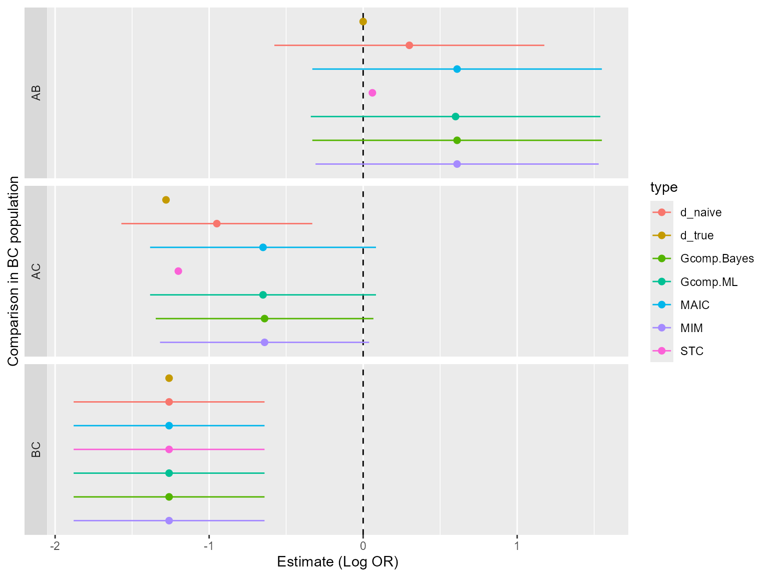
We now combine all outputs and present in plots and tables. For a log-odds ratio a table of all contrasts and methods in the $BC$ population is given below.

	d_true	d_naive	MAIC	STC	Gcomp.ML	Gcomp.Bayes	MIM
AB	0.00	0.30	0.61	0.06	0.60	0.61	0.61
AC	-1.28	-0.95	-0.65	-1.20	-0.65	-0.64	-0.64
BC	-1.26	-1.26	-1.26	-1.26	-1.26	-1.26	-1.26

We can see that the different corresponds reasonably well with one another.

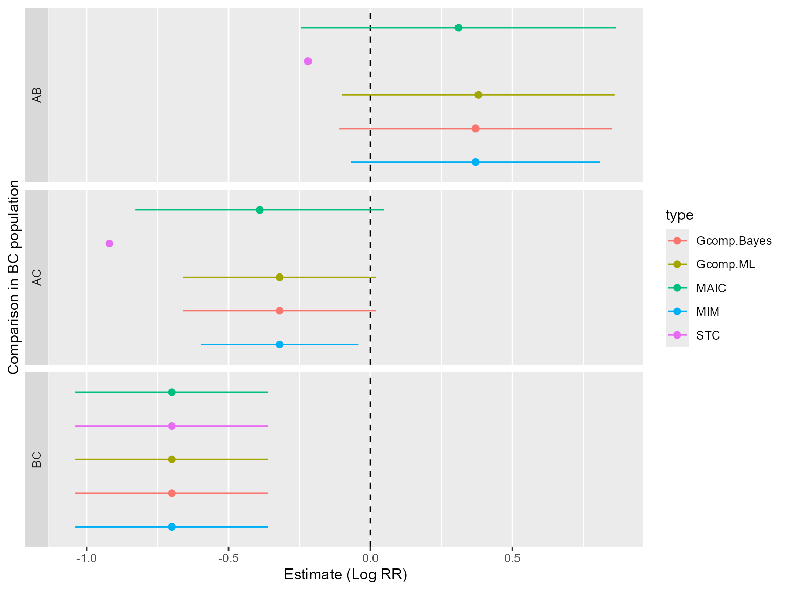
Next, let us look at the results on the log relative risk scale. First, the true values are calculated as

d_AB_true_lrr <- 0
d_AC_true_lrr <- log(plogis(d_A_true) / plogis(d_C_true))
d_AC_true_lrr

so that the summary table is

	MAIC	STC	Gcomp.ML	Gcomp.Bayes	MIM
AB	0.31	-0.22	0.38	0.37	0.37
AC	-0.39	-0.92	-0.32	-0.32	-0.32
BC	-0.70	-0.70	-0.70	-0.70	-0.70

Plots

The same output can be presented in forest plots is as follows. Each horizontal bar represent a different method and the facets group these by treatment comparison for the $BC$ population. The log-odds ratio and log risk ratio plot are given below.